Record a Macro in Excel to Fix an Imported Text File

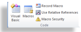
Macro Commands

Macro Commands

A viewer asked for my help in fixing a “Text” file that he imports into Excel each month. His IT department creates this file for him. The problem is that:

  • The Field Header Labels are arranged on two rows – He needs all of the labels to be on one row.
  • Each record is arranged on two rows – He needs each record to appear on one row.
  • There is a blank row separating each record  – He needs to remove all of the blank rows.

This is a perfect job for an Excel Macro!

In this tutorial, I first demonstrate how to create the Macro in Excel 2010. Then, I repeat the process using Excel 2003 – the version that my viewer is currently using.

Topics Covered in the Tutorial

  • Adding the Developer Tab to the Ribbon in Excel 2010
  • Creating back up copies of worksheets before recording the Macro
  • Using the Fill Across Worksheets (Grouped) to copy both content and formatting
  • Using Relative References when Recording a Macro
  • Planning the steps you will take before Recording the Macro
  • Using Keyboard Shortcuts to Run the Macro
  • Creating and Editing a Command Button to Run the Macro
  • Viewing the VBA Code that Excel creates when you Record the Macro
  • Using Step Into to see how each step in the Macro is executed
  • Viewing and Changing Security Settings for Macros
  • Storing Macros in a Trusted Location (Excel 2007 and Excel 2010)
  • Saving Worksheets that contain Macros in Excel 2007 and Excel 2010

Watch Tutorial in High Definition

Follow this link to view this Excel Tutorial in High Definition mode on my YouTube Channel – DannyRocksExcels.
Share and Enjoy:
  • Add to favorites
  • Facebook
  • Twitter
  • Technorati
  • Print
  • email
  • Digg
  • StumbleUpon
  • del.icio.us
  • Yahoo! Buzz
  • Google Bookmarks
  • Orkut
  • SphereIt
  • Sphinn

Create a Custom Excel Function to Replace Formulas with Multiple IF Functions

Multiple Nested IF Functions

Multiple Nested IF Functions

Do you get tied up in a knot trying to write – let alone explain – a formula that has one IF Function nested inside another, and another…? I know that I do! And, what happens when your sales manager wants to revise the tiers for the quantity discounts? How many hours will this take you to review your logic and to make all of those multiple changes?

Usually, this will mean a lot of time, a lot of frustration and possibly some resentment thrown in as well!

Well, relax. I am going to demonstrate how easy it is to write a custom function in Excel using the “Select Case” Construct to replace the “rat’s nest” of multiple IF Functions in your formulas!

Scenario for this Function

You have been asked by your Sales Manager to write a formula to grant a discount, based upon the quantity of units ordered. There are 5 Tiers: Below 5 units ordered, no discount. From 6 to 24 units, a 10% discount, etc. Rather than spending a half hour nesting IF() functions and using AND() functions to create this formula, spend less than 10 minutes creating a Custom Excel Function instead.

Create the Custom Excel Function

  • Begin by opening the Visual Basic Editor. One way to do this is right-click any worksheet tab and select “View Code.”
  • Ensure that you have inserted a Module in the Project Explorer and that you have selected the module.
  • In the example that I use on this video tutorial, my first line of code is: “Function DiscQty(quantity)” and this is matched to an “End Function” statement
  • For this Custom Function, I am using the “Select Case” Construct in Visual Basic (VBA). Think of the keyword “Case” as a substitute for the =IF() Function.
  •  Rather than nesting the Excel =AND() Function inside the IF() Function, you will substitute – e.g. “Case 6 To 24” and then “DiscQty = 0.1” to indicate a 10% discount for quantities between 6 AND 24.

Watch the video to see how easy is is to create – and use – this custom Excel function. Invest the 7 minutes and 47 seconds to watch it – I guarantee that this investment of time will pay you many dividends for years and years to come!

View This Video Tutorial in High Definition

Follow this link to watch this Excel Video Tutorial in High Definition on my YouTube Channel – DannyRocksExcels.

Share and Enjoy:
  • Add to favorites
  • Facebook
  • Twitter
  • Technorati
  • Print
  • email
  • Digg
  • StumbleUpon
  • del.icio.us
  • Yahoo! Buzz
  • Google Bookmarks
  • Orkut
  • SphereIt
  • Sphinn

Write an Excel Macro in VBA to Update Worksheet Tab Name

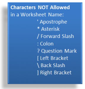
Characters Not Allowed in Worksheet Names

Characters Not Allowed in Worksheet Names

This is Part 2 of my two-part series of video tutorials where I demonstrate how to link an Excel Worksheet Tab Name and the contents of a Worksheet Cell.

In this lesson, I show you how to write an Excel Macro in VBA (Visual Basic for Applications) that will update the name of the Worksheet Tab based on the value of a cell in that worksheet.

Write Excel Macro in VBA

For this Macro, the first line of code will prevent the Macro from crashing if the cell contains one of the “disallowed” characters that you see in the diagram

On Error Resume Next

The second line of code initiates a “For – Next” loop of instruction

For Each ws In Thisworkbook.Worksheets

The third line of code is the Instruction to follow in the “For – Next” Loop

ws.Name = Left(ws.Cells(1,5).Value, 31)

Here, this instruction is saying – in plain English – “Nane this Worksheet (ws) using the leftmost 31 characters in the cell that is in the 1st row of the 5th column – (Cell E1)”

The reason for including 31, is that that is the maximum number of characters allowed in an Excel Worksheet Tab Name.

The fourth and fifth lines of code complete the macro – watch the video to see what they are (What a “tease” I am!!)

Run Macro from Command Button

In this lesson I also show you how to run this Macro from a command button that I add to the Quick Access Toolbar in Excel 2007 or Excel 2010.

Watch Video in High Definition on YouTube

 Click on this link to watch this Excel Video Tutorial in High Definition on my YouTube Channel – DannyRocksExcels

Source for This Code

I found the code for this example in one of Bill Jelen, Mr. Excel’s Books, “Excel Gurus Gone Wild.”

Bill’s website is: http://www.mrexcel.com/

Watch Part 1 of this Series

Here is the link to Part 1 of this series. I show you how to write a Custom Excel Function to insert the Name of the Worksheet Tab into a cell on the worksheet.

Share and Enjoy:
  • Add to favorites
  • Facebook
  • Twitter
  • Technorati
  • Print
  • email
  • Digg
  • StumbleUpon
  • del.icio.us
  • Yahoo! Buzz
  • Google Bookmarks
  • Orkut
  • SphereIt
  • Sphinn

How to Use an Excel Macro to Quickly Fill in Blank Cell Labels

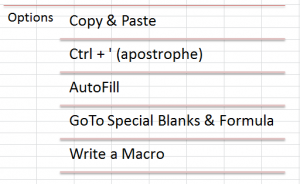
Options for Filling in Blank Cell Labels

Options for Filling in Blank Cell Labels

In this Excel video tutorial, I demonstrate how to write, proofreed and run a Macro that will quickly fill in values for blank cell lables in a report that you may have received from a colleague or a client.

Reports With “Holes in the Data”

Frequently, when you receive a report that was created in an Excel Pivot Table or from a relational database – e.g. MS Access – the report looks great! However, if you wish to apply filters or other analysis to this report, you will need to fill in the “missing” or blank cell labels.  

Watch This Excel Video Tutorial in High Definition

Follow this link to view this lesson in High Definition, Full Screen Mode on my YouTube Channel – DannyRocksExcels

Related Excel Video Tutorials

If you would like to learn how to convert an Excel Pivot Table to a Standard List – and to Fill in the Blank Cell Labels – click on this link to see my video tutorial on this topic.

And, here is a link to another related Excel Video Tutorial – Quickly Fill in Blank Cell Labels

Share and Enjoy:
  • Add to favorites
  • Facebook
  • Twitter
  • Technorati
  • Print
  • email
  • Digg
  • StumbleUpon
  • del.icio.us
  • Yahoo! Buzz
  • Google Bookmarks
  • Orkut
  • SphereIt
  • Sphinn