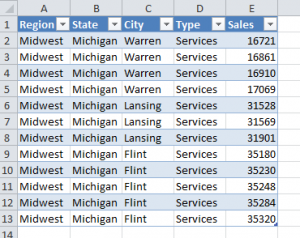
How to Drill Down in a Pivot Table to Display the Details for a Summary Cell

Drill Down Details in Pivot Table

Excel Pivot Table Reports are a great way to summarize the results of multiple records in an underlying data set.

However, at some point, someone will question the accuracy of a specific calculation in your Pivot Table – this is to be expected.

When this happens. you can quickly “drill down” to display the details for any summary cell in your Pivot Table. You simply “double-click” the summary cell and you get to review the detail on a new worksheet in your Excel workbook.

Refreshing a Pivot Table

The key points to understand about Excel Pivot Tables are:

You cannot change an individual value in a Pivot Table.
You cannot update any changes from a “drill down” worksheet in a Pivot Table.
After you edit your underlying data set, you must “Refresh” your Pivot Table to get the revised calculations.

Formatting “Blank Cells” in a Pivot Table

One aspect of Pivot Tables – displaying “blank cells” – is disconcerting to many people who are using or viewing Pivot Tables for the first time. In this video tutorial, I demonstrate how to customize the display of these cells that have no underlying values to calculate.