Working with Custom Lists in All Versions of Excel

Edit Custom Lists in Excel

Edit Custom Lists in Excel

Custom Lists in Excel are great because the help to ensure accuracy and consistency when entering data on a worksheet. Excel comes with several Custom Lists built-in to the program – e.g. Days of the Week and Months of the Year. Now, you can quickly use Excel’s AutoFill handle to add Jan, Feb, Mar, Apr, etc. in any direction (vertical or horizontal) on the active worksheet.

Edit Custom Lists

You can quickly create – or edit – your own Custom List. Follow these steps:

  1. Type your list in a contiguous group of cells – either vertically or horizontally.
  2. Select the cells with the values that you just entered.
  3. Spell check this list – use the F7 Keyboard Shortcut
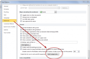
  4. Open up the Edit Custom List Dialog Box. (Watch this video to see how this is differs between Excel 2010, Excel 2007 and Excel 2003.)
  5. With your new Custom List selected, click the “Import” button to add your Custom List to the current version of Excel on this computer.

Sort Data Using a Custom List

On this video tutorial, I demonstrate how to sort a list of data using a Custom List – e.g. to get the “Month” field sorted in chronological order (January, February, etc.) This will save you a great deal of time!

Create a Custom List for Letters of Alphabet

Having a Custom List for the 26 letters of the alphabet comes in handy on many occasions. I show you how to AutoFill down the initial list using =Char(Row() + 64) beginning in Row 1 – a really usefuly function!

View This Excel Video Tutorial in High Definition

Follow this link to watch this video tutorial in High Definition on my YouTube Channel – DannyRocksExcels

Get my best-selling DVD-ROM, “The 50 Best Tips for Excel 2007” for only $29.97!

How to Embed an Interactive Excel Workbook from a Sky Drive in Windows Office Live!

For the past two or three months, I have been uploading the Excel Workbooks that I use during my video tutorials to my Sky Drive at Windows Office Live! – www.office.live.com Just this past week, I learned that I can also “embed” those stored files here – in a blog post – on my website! So, here is my first attempt to share an “interactive Excel Workbook” with you.

Embedded Excel Workbook

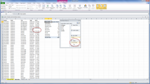
This Excel worksheet is one of the basic data sets that I use when I demonstrate how to create Excel Pivot Tables. Scroll horizontally or vertically to see the Pivot Table. Notice that you can use the drop-down filters in the Pivot Table!

Click the Icon in the lower right corner of the Excel WebApps frame and you will be taken to my Sky Drive online where you can view or manipulate the worksheet in Full Screen More. Or, you can choose to download this file to your computer to work on it with the full range of Excel commands.

Download Excel Video Tutorial Recordings for $9.95

If you want to learn more about Pivot Tables, click on this link to gather information on my new series of Extended Length (one hour +) Excel Video Tutorials. You can download these videos to your computer for only US $9.95 from my WebEx by Cisco site – http://thecompanyrocks.webex.com – I store all of the Excel Workbooks that I use in the lessons on my Sky Drive online!

Watch This Video Tutorial in High Definition on YouTube

Follow this link to watch my step-by-step instructions to accomplish this task – in High Definition – on my YouTube Channel, DannyRocksExcels.

How a Single Blank Cell Affects an Excel Pivot Table Report

As you will see in this Excel Video Tutorial, having a single blank cell in a data set will greatly affect how Excel Functions and Pivot Tables are designed and calculated.

Single Blank Cell in Data

Single Blank Cell in Data

Imagine, how a single blank cell, in a field of 848 records, can change the way your Pivot Table views the data type (text vs. the expected numeric data type) and subtotal function (Count vs. the expected SUM function).

Seeing is believing!

Preventing a Blank Cell from “Creeping into” your data set

Use the Keyboard Shortcut Ctrl + Down Directional Arrow to go to the last cell that contains data in a column. This is a great way to isolate “stray” blank cells that will have a great impact on your Pivot Tables and other calculations in Excel.

Also, in Excel 2007 and Excel 2010, look for where a “numeric” field is placed by default. A single blank cell will cause an (intended) numeric field to be placed in the Row (text) labels area. Even dragging this field into the VALUES Drop zone does not solve the problem because the COUNT Function will be used to Subtotal this field. This is a “disaster waiting to happen!”

Introducing My Extended Length Excel Video Recordings

This is my opportunity to introduce you to my new, extended-length (one-hour +) Excel Video Tutorials that you can download for only US $9.95!

Here is the link that gives you more information about this exciting new service:

http://www.thecompanyrocks.com/pivot-table-tutorial-videos-to-download-practice-files-instructional-manual-included/

I offer you multiple options:

Let me know what you think!

Let me know which topics you would like me to record for you to download.

Send me an email with your comments and suggestions: danny@thecompanyrocks.com

Watch This Video in High Definition

Follow this link to view this Excel Tutorial in High Definition on my YouTube Channel – DannyRocksExcels

Create a Custom Excel Function to Replace Formulas with Multiple IF Functions

Multiple Nested IF Functions

Multiple Nested IF Functions

Do you get tied up in a knot trying to write – let alone explain – a formula that has one IF Function nested inside another, and another…? I know that I do! And, what happens when your sales manager wants to revise the tiers for the quantity discounts? How many hours will this take you to review your logic and to make all of those multiple changes?

Usually, this will mean a lot of time, a lot of frustration and possibly some resentment thrown in as well!

Well, relax. I am going to demonstrate how easy it is to write a custom function in Excel using the “Select Case” Construct to replace the “rat’s nest” of multiple IF Functions in your formulas!

Scenario for this Function

You have been asked by your Sales Manager to write a formula to grant a discount, based upon the quantity of units ordered. There are 5 Tiers: Below 5 units ordered, no discount. From 6 to 24 units, a 10% discount, etc. Rather than spending a half hour nesting IF() functions and using AND() functions to create this formula, spend less than 10 minutes creating a Custom Excel Function instead.

Create the Custom Excel Function

  • Begin by opening the Visual Basic Editor. One way to do this is right-click any worksheet tab and select “View Code.”
  • Ensure that you have inserted a Module in the Project Explorer and that you have selected the module.
  • In the example that I use on this video tutorial, my first line of code is: “Function DiscQty(quantity)” and this is matched to an “End Function” statement
  • For this Custom Function, I am using the “Select Case” Construct in Visual Basic (VBA). Think of the keyword “Case” as a substitute for the =IF() Function.
  •  Rather than nesting the Excel =AND() Function inside the IF() Function, you will substitute – e.g. “Case 6 To 24” and then “DiscQty = 0.1” to indicate a 10% discount for quantities between 6 AND 24.

Watch the video to see how easy is is to create – and use – this custom Excel function. Invest the 7 minutes and 47 seconds to watch it – I guarantee that this investment of time will pay you many dividends for years and years to come!

View This Video Tutorial in High Definition

Follow this link to watch this Excel Video Tutorial in High Definition on my YouTube Channel – DannyRocksExcels.

Write an Excel Macro in VBA to Update Worksheet Tab Name

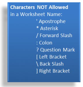
Characters Not Allowed in Worksheet Names

Characters Not Allowed in Worksheet Names

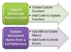
This is Part 2 of my two-part series of video tutorials where I demonstrate how to link an Excel Worksheet Tab Name and the contents of a Worksheet Cell.

In this lesson, I show you how to write an Excel Macro in VBA (Visual Basic for Applications) that will update the name of the Worksheet Tab based on the value of a cell in that worksheet.

Write Excel Macro in VBA

For this Macro, the first line of code will prevent the Macro from crashing if the cell contains one of the “disallowed” characters that you see in the diagram

On Error Resume Next

The second line of code initiates a “For – Next” loop of instruction

For Each ws In Thisworkbook.Worksheets

The third line of code is the Instruction to follow in the “For – Next” Loop

ws.Name = Left(ws.Cells(1,5).Value, 31)

Here, this instruction is saying – in plain English – “Nane this Worksheet (ws) using the leftmost 31 characters in the cell that is in the 1st row of the 5th column – (Cell E1)”

The reason for including 31, is that that is the maximum number of characters allowed in an Excel Worksheet Tab Name.

The fourth and fifth lines of code complete the macro – watch the video to see what they are (What a “tease” I am!!)

Run Macro from Command Button

In this lesson I also show you how to run this Macro from a command button that I add to the Quick Access Toolbar in Excel 2007 or Excel 2010.

Watch Video in High Definition on YouTube

 Click on this link to watch this Excel Video Tutorial in High Definition on my YouTube Channel – DannyRocksExcels

Source for This Code

I found the code for this example in one of Bill Jelen, Mr. Excel’s Books, “Excel Gurus Gone Wild.”

Bill’s website is: http://www.mrexcel.com/

Watch Part 1 of this Series

Here is the link to Part 1 of this series. I show you how to write a Custom Excel Function to insert the Name of the Worksheet Tab into a cell on the worksheet.

Write a Custom Excel Function to Link Worksheet Tab Name to a Cell

Custom Functions in Excel

Custom Excel Functions

In response to many viewer requests, I am creating a two-part series of video tutorials that show you how to create links between the name of an Excel Worksheet Tab and a cell on that worksheet.

Here, in Part One, I demonstrate how to write a Custom Excel Function to capture the name of the worksheet tab in a cell.

Write Custom Excel Functions

You write Custom Excel Functions in the Visual Basic Editor. One way to open the Visual Basic Editor is to use the keyboard shortcut Alt + F11. Here are the elements that I use in this lesson:

  • Open the Project Explorer Pane (Keyboard Shortcut Ctrl + R).
  • Insert a Module to contain the VBA Code that you write for your Custom Function
  • Open the Code Pane (Keyboard Shortcut F7).

Write the Code for the Custom Function

In its simplest form, this is all of the code that you need for this Custom Excel Function:

Function SHEETNAME2() As String
SHEETNAME2 = Application.Caller. Parent.Name
End Function


That’s it!

Automatically Update Results of Custom Functions

A major difference between Custom Functions that you write and Excel’s Built-in Functions is that by default, the result of a Custom Function does not automatically update when values or references change. If you want your Custom Function to automatically update whenever the worksheet changes, add this line of code to your Custom Function in the Module:

Application.Volatile True

Source for this Code

I found the code for this Custom Excel Function in John Walkenbach’s Book, “Excel 2007 Formulas. He is an Excel Expert and I admire his writing style. You can check out his reources at this site:

http://spreadsheetpage.com/

Watch this Video in High Definition on YouTube

Click on this link to view this Excel Tutorial on my YouTube Channel – DannyRocksExcels.

Watch Part 2 of This Series

Here is the link to Part 2 in this Series. In this lesson I show you how to write an Excel Macro in VBA to update the Name of the Worksheet Tab based upon the value in a cell on the worksheet.

How to Use an Excel Macro to Quickly Fill in Blank Cell Labels

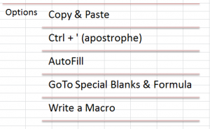
Options for Filling in Blank Cell Labels

Options for Filling in Blank Cell Labels

In this Excel video tutorial, I demonstrate how to write, proofreed and run a Macro that will quickly fill in values for blank cell lables in a report that you may have received from a colleague or a client.

Reports With “Holes in the Data”

Frequently, when you receive a report that was created in an Excel Pivot Table or from a relational database – e.g. MS Access – the report looks great! However, if you wish to apply filters or other analysis to this report, you will need to fill in the “missing” or blank cell labels.  

Watch This Excel Video Tutorial in High Definition

Follow this link to view this lesson in High Definition, Full Screen Mode on my YouTube Channel – DannyRocksExcels

Related Excel Video Tutorials

If you would like to learn how to convert an Excel Pivot Table to a Standard List – and to Fill in the Blank Cell Labels – click on this link to see my video tutorial on this topic.

And, here is a link to another related Excel Video Tutorial – Quickly Fill in Blank Cell Labels

How to Take Advantage of Excel 2007 – 2010 Tables and Excel 2003 Lists

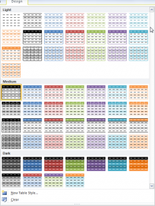
Excel Table Styles

Excel Table Styles

In this video tutorial, I cover multiple versions of Excel. I demonstrate how to take advantage of the Table Tools that were introduced in Excel 2007 and I also show you how to create Excel 2003 Lists.

Topics Covered on Video Tutorial

  • Convert a range of data to an Excel 2007, Excel 2010 Table.
  • Convert a range of data to an Excel 2003 List.
  • View and change the Total Row in each version of Excel.
  • Append new records to Tables and Lists.
  • Add a new field to Tables and Lists.
  • Write a formula in one cell of an Excel Table and have it automatically copy down for each record.
  • Change the Table Styles in Excel 2007 and 2010.
  • Use Conditional Formatting to add alternate row shading to an Excel 2003 List

Watch Video in High Definition on YouTube

Follow this link to watch this Excel Video Tutorial in High Definition on my YouTube Channel, DannyRocksExcels

Download This Excel Workbook

Click on this link to download the Excel Workbook that I used in this video tutorial.

Get my best-selling DVD-ROM, “The 50 Best Tips for Excel 2007” for only $39.95!

Refer to an Excel Table Field When Writing Formulas

Refer to Excel Table in Formula

Refer to Excel Table in Formula

While I strongly recommend creating “Named Ranges” that you can refer to in an Excel Formula, there is one drawback. By default, “named ranges” refer to “Absolute” Cells – e.g. $A$1:$A$15

However, what happens when your data set expands? For example, when you add records beyond row 15 in this case.  Now, your formulas do not refer to the additional data in each field. You need to find a way to automatically expand the range of cells that your formula refers to.

Tables in Excel 2007 and Excel 2010

Fortunately, if you are using either Excel 2007 or Excel 2010, you can “format” your data set as an EXCEL TABLE and take advantage of many great options:

  • When you append records (rows) , the definition of your Table automatically expands.
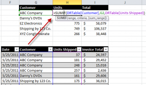
  • You can “name” your table to reflect its contents. For example, in this video I name my Table – DRTable –  and I refer to it in my formulas.

Writing Formulas that Refer to Excel Table Field

In this video tutorial I use the SUMIF Function. Remember that I have “named”my table DRTable. Here is how I begin my formula. =SUMIF(DRTable[Customer]. Notice the use of brackets ([ ]) around the [Customer] Field in the formula. This is the gotcha step in this lesson.

Watch This Video in High Definition on YouTube

I created this video tutorial in High Definition Mode. Click on this link to view it on my YouTube Channel – DannyRocksExcels

Get my best-selling DVD-ROM, “The 50 Best Tips for Excel 2007” – Visit my Online Bookstore for more information.

How to Maintain Accurate Subtotals When Your Data Set Expands in Size

Subtotal in Excel 2010 Table

Subtotal in Excel 2010 Table

This is Part 2 of my series of video tutorials demonstrating how to use the SUBTOTAL Function in Excel.

  • In Part 1, I showed you the value of using the Subtotal Function to summarize the results of applying a Data Filter to a range of cells.
  • In this part, I show you how to use an Excel 2007 or Excel 2010 Table to ensure that your Subtotal Formulas are automatically updated when you append records or add additional fields to your original data set.

I strongly recommend basing Filtered Lists and Pivot Tables on an Excel Table (in Excel 2007 or 2010) or an Excel List in Excel 2003. This way, any formulas, filters and references that you make will be automatically updated when you append additional records or otherwise change the structure of your data set.

Function Numbers 101 through 111

Notice that when you “toggle on” the Total Row for a Table or List that Excel uses this formula = SUBTOTAL(109, Table1, [Sales]). Function 109 will use the SUM Function(109) to total the values in the “Sales” field ([Sales]) of a Table named “Table1.” These Function Numbers + 100 were introduced in Excel 2003 and the are automatically applied whenever you are using a Total Row in an Excel Table.

I think that you will learn some cool tricks in this lesson. Let me know what you think!

Watch This Video in High Definition

Click on this link to watch this video tutorial in High Definition, Full Screen Mode on my YouTube Channel – DannyRocksExcels.

Invitation to Visit My New Online Shopping Site

I invite you to visit my new, secure online shopping website – http://shop.thecompanyrocks.com

Once there, you can get my best-selling DVD-ROM, “The 50 Best Tips for Excel 2007”