How to Use the SOLVER Tool in Excel to Produce the Optimal Result for a Formula

Key Points for SOLVER

SOLVER in Excel – Key Points

I am responding to a “flurry” of requests to produce an Excel Video Tutorial that demonstrates how to use the SOLVER TOOL in Excel. Here are the key points to remember when you want to use the SOLVER Tool:

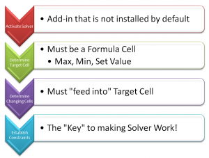
Activate the SOLVER Tool

SOLVER is an “Add-in” tool that needs to be “activated” before you can use it. In Excel 2007 / 2010, you do this via Excel Options – Addi-Ins – Excel Options. In Excel 2003, you do this via the Tools Menu – Add-ins – Solver.

Prepare Data for Solver

In order to use the SOLVER Tool, you must:

  • Establish the “Target Cell.” This cell must contain a formula. This is the cell that you want to “optimize” by using SOLVER.
  • Determine the “By Changing” Cells. These are the cells that SOLVER will change in order to deliver the optimized result in the Target Cell. The “By Changing” cells MUST “Feed Into” the Target Cell.
  • Establish the CONSTRAINTS for SOLVER. This is the “key’ element that gives SOLVER its power. You can add as many constraints as needed. My recommendation is that you “write them out” before you start  to use the SOLVER Tool.

SOLVER is very powerful. However, you MUST “think it through” before you apply it. It will take lots of practice for you to understand how to properly set up your data to produce appropriate SOLVER results.

Part 2 in this Series of Tutorials for Solver in Excel

Here is the link to watch Part 2 in this Series of Tutorials about the SOLVER Add-in Tool in Excel

Download Excel Workbook for this Lesson

Follow this link to download the Excel Workbook that I used for this lesson. I store my uploaded Excel workbooks on my SkyDrive at www.office.live.com

View this Tutorial in High Definition

Click on this link to watch this Excel Tutorial in High definition / Full Screen Mode – on my YouTube Channel, DannyRocksExcels
Share and Enjoy:
  • Add to favorites
  • Facebook
  • Twitter
  • Technorati
  • Print
  • email
  • Digg
  • StumbleUpon
  • del.icio.us
  • Yahoo! Buzz
  • Google Bookmarks
  • Orkut
  • SphereIt
  • Sphinn

How to Embed an Interactive Excel Workbook from a Sky Drive in Windows Office Live!

For the past two or three months, I have been uploading the Excel Workbooks that I use during my video tutorials to my Sky Drive at Windows Office Live! – www.office.live.com Just this past week, I learned that I can also “embed” those stored files here – in a blog post – on my website! So, here is my first attempt to share an “interactive Excel Workbook” with you.

Embedded Excel Workbook

This Excel worksheet is one of the basic data sets that I use when I demonstrate how to create Excel Pivot Tables. Scroll horizontally or vertically to see the Pivot Table. Notice that you can use the drop-down filters in the Pivot Table!

Click the Icon in the lower right corner of the Excel WebApps frame and you will be taken to my Sky Drive online where you can view or manipulate the worksheet in Full Screen More. Or, you can choose to download this file to your computer to work on it with the full range of Excel commands.

Download Excel Video Tutorial Recordings for $9.95

If you want to learn more about Pivot Tables, click on this link to gather information on my new series of Extended Length (one hour +) Excel Video Tutorials. You can download these videos to your computer for only US $9.95 from my WebEx by Cisco site – http://thecompanyrocks.webex.com – I store all of the Excel Workbooks that I use in the lessons on my Sky Drive online!

Watch This Video Tutorial in High Definition on YouTube

Follow this link to watch my step-by-step instructions to accomplish this task – in High Definition – on my YouTube Channel, DannyRocksExcels.

Share and Enjoy:
  • Add to favorites
  • Facebook
  • Twitter
  • Technorati
  • Print
  • email
  • Digg
  • StumbleUpon
  • del.icio.us
  • Yahoo! Buzz
  • Google Bookmarks
  • Orkut
  • SphereIt
  • Sphinn

How to Take Advantage of Excel 2007 – 2010 Tables and Excel 2003 Lists

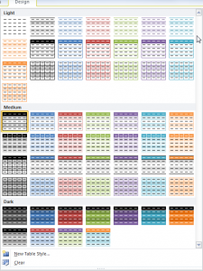
Excel Table Styles

Excel Table Styles

In this video tutorial, I cover multiple versions of Excel. I demonstrate how to take advantage of the Table Tools that were introduced in Excel 2007 and I also show you how to create Excel 2003 Lists.

Topics Covered on Video Tutorial

  • Convert a range of data to an Excel 2007, Excel 2010 Table.
  • Convert a range of data to an Excel 2003 List.
  • View and change the Total Row in each version of Excel.
  • Append new records to Tables and Lists.
  • Add a new field to Tables and Lists.
  • Write a formula in one cell of an Excel Table and have it automatically copy down for each record.
  • Change the Table Styles in Excel 2007 and 2010.
  • Use Conditional Formatting to add alternate row shading to an Excel 2003 List

Watch Video in High Definition on YouTube

Follow this link to watch this Excel Video Tutorial in High Definition on my YouTube Channel, DannyRocksExcels

Download This Excel Workbook

Click on this link to download the Excel Workbook that I used in this video tutorial.

Get my best-selling DVD-ROM, “The 50 Best Tips for Excel 2007” for only $39.95!

Share and Enjoy:
  • Add to favorites
  • Facebook
  • Twitter
  • Technorati
  • Print
  • email
  • Digg
  • StumbleUpon
  • del.icio.us
  • Yahoo! Buzz
  • Google Bookmarks
  • Orkut
  • SphereIt
  • Sphinn

Two Ways to Turn Excel Data On Its Side – Transpose the Data!

Transpose Excel Data

Transpose Excel Data

How many times have you spent an hour or more creating an Excel worksheet only to discover – or be told – that you have the wrong structure? The values that you entered run vertically down in Column A. And  now, you need to have your values run horizontally across in Row 1.

Well, don’t despair! And, most important, do NOT retype your entries on another worksheet. Rather,watch this video to see how to “Turn Excel Data On Its Side”:

  1. Select Transpose from the Paste Select dialog box or the right-click shortcut menu
  2. Use the =TRANSPOSE() Function which is an Array Function

Watch as I demonstrate the advantages of each approach – they are different! If you are “curious” about how an Array Function works, the TRANSPOSE Function is a good one to practice with.

Click this link to watch this video in High Definition on YouTube.

Now Using Excel 2010

I filmed this video using Excel 2010. I will use Excel 2010 for all future video lessons unless there is a particular need to use another version to illustrate a point.

Download Workbook Used in This Video

Click on this link to download the Excel Workbook that I used in this video tutorial. It is stored on my “SkyDrive” at www.office.live.com

Get my best-selling DVD-ROM, “The 50 Best Tips for Excel 2007” for only $29.97!

Share and Enjoy:
  • Add to favorites
  • Facebook
  • Twitter
  • Technorati
  • Print
  • email
  • Digg
  • StumbleUpon
  • del.icio.us
  • Yahoo! Buzz
  • Google Bookmarks
  • Orkut
  • SphereIt
  • Sphinn

How to Create an Interactive Pivot Chart in Excel

While I have created many Excel Video Tutorials demonstrating the power of interactive Pivot Tables during the past four years, I have NEVER created a video lesson focused on creating interactive Pivot Charts in Excel – until now!

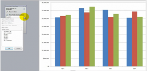
Interactive Pivot Table Chart

Interactive Pivot Table Chart

Pivot Charts in Excel 2007

In this lesson, I show you how to create a Pivot Chart in Excel 2007. Starting with Excel 2007, there are several major changes:

  • By default, Pivot Charts are embedded on the same worksheet as the Pivot Table Report that is linked to the chart.
  • A new, PivotTable Chart Filter Dialog box is available – this works “in tandem” with the filters available in the PivotTable Field List” Dialog box.
  • It is very easy to “Move” a Pivot Chart to its own worksheet tab – or vice versa – to move the Pivot Chart to an existing worksheet.

 Pivot Charts and Pivot Table Reports are Connected

A Pivot Chart MUST be connected to a Pivot Table Report. Any changes that you make to the chart are reflected in the report and vice versa. If you filter the Pivot Table Report, the filter is automatically applied to the Pivot Chart. This is an important concept to understand. This is the reason why it is so easy to make BOTH Pivot Table Reports and Pivot Charts “interactive!”

Explore My Index of Free Excel Video Lessons

I was surprised to discover that I had not yet created a video tutorial for Excel Pivot Charts when I looked at my list of “free” Excel Video Lessons. This became the impetus for creating this lesson. I invite you to explore all of my free Excel Video Tutorials. Click on this link to go to my Index of Excel Video Lessons. I have organized the free video lessons by topic. Simply click on the title of any lesson and you will arrive at the posting and the video for that lesson.

Download Excel File for This Lesson

View this Lesson in High Definition

I invite you to view this Excel Video Tutorial in High Definition, Full-screen Mode on my YouTube Channel – DannyRocksExcel

Watch Video Now


Feedback Welcome

I always welcome your feedback. Let me know what you think about this – or any other – video lesson. Add your comments below!

Extended Length Video Training Resource for Pivot Tables

I have created 90-minutes video training resources for Pivot Tables. Follow this link to learn more about my “Master Excel in Minutes” series.

Share and Enjoy:
  • Add to favorites
  • Facebook
  • Twitter
  • Technorati
  • Print
  • email
  • Digg
  • StumbleUpon
  • del.icio.us
  • Yahoo! Buzz
  • Google Bookmarks
  • Orkut
  • SphereIt
  • Sphinn

Download My Excel Workbooks and Step-by-Step Instructional Manuals for Free!

Finally! I have figured out a way to allow my viewers to download the Excel Workbooks, Word Documents, PowerPoint Presentations, etc. that I use in my video lessons. For the past few months, I have been able to give you a direct link to download the Adobe Acrobat files that I create. For example:

My problem has been that – Starting in Office 2007 –  the underlying file structure of each program (Excel, Word, PowerPoint, etc.) has changed and it is no longer possible to “Publish to the Web” the worksheets, documents and presentations that I offered in the past. I will spare you the boring details of why and how this has happened, because I have good news for you!

Enter, “The Cloud!”

Cloud Computing

You have probably seen or heard this advertising slogan recently. Here is how I have just discovered how “The Cloud” can work for both you and me:

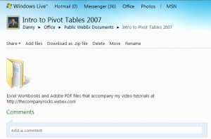
Initially, I am uploading – and sharing – the workbooks, documents, PDFs, etc. that accompany the extended video recordings that I offer on my http://thecompanyrocks.webex.com site.

This is a new development for me and The Company Rocks. I offer a series of extended length ( 25 minute to 60 minutes) video tutorials.

  • Intro to Pivot Tables in Excel 2007

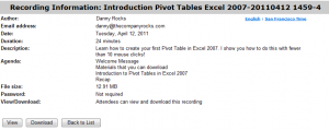
    Information about this Video Recording


  • As I write this posting, I have 4 modules – each offered “free of charge” – for you to view and / or download.
  •  
  •  

Go to http://thecompanyrocks.webex.com to see what I currently offer you!

  • As I gather feedback, activity, statistics, etc. I may extend the range of downloadable content that I create – My decision will depend upon your feedback, so please add your comments below in this posting!
  • My Next Level of Product Offerings 

    I am on a journey to evolve the range and detail of the products and services that I offer you, my loyal viewers and subscribers. I wnat to be responsive to your needs. So, that meanrs that the more feedback that I get from you – my viewers and subscribers – the better I can structure my offerings. I welcome your feedback!

    Based on some great feedback from my viewers and subscribers, I have just begun to create a series of extended length ( 25 to 45 minutes) video tutorials. The initial tutorials will be offered “free of charge.” Other video tutorials will be carry a modest – I might add, aggressive – pricing model! My goal is to give you the product and content that you need at a price that is mutually acceptable! You, and your level of supposrt will tell me what is acceptable – please give me your feedback!

    Extended Video Tutorials Now Online

    You can now view or download – after registering – at WebEx by Cisco – for these video tutorials that I have posted:


    I hope that you find these links and videos helpful. Please add your feeback via the comments section below this post.

    Sincerely,

    Danny Rocks

    www.thecompanyrocks.com

    Share and Enjoy:
    • Add to favorites
    • Facebook
    • Twitter
    • Technorati
    • Print
    • email
    • Digg
    • StumbleUpon
    • del.icio.us
    • Yahoo! Buzz
    • Google Bookmarks
    • Orkut
    • SphereIt
    • Sphinn

    Functions to Analyze Loan Payments in Excel

    Loan Payment Functions

    Loan Payment Functions

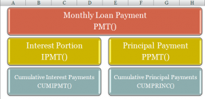
    When you use the PMT Function in Excel, the result is the amount of money that you will pay each period (usually monthly) until the loan is repaid. When you want to know how much of each payment is an interest charge, you use the IPMT Function. And,to find the amount that goes towards reducing the principal on your loan, you use the PPMT Function.

    Cumulative Payments

    Two other functions are helpful in analyzing your loan payments. When you want to see the Cumulative amount of Interest (CUMIPMT Function) that you paid between two periods – e.g. Starting with payment 1  and ending with payment 12. You use the CUMPRINC Function to total the amount of your loan payments that went towards reducing the principal on your loan between any two periods.

    Absolute and Relative Cell References

    As you will see in the video, I use a combination of Absolute Cell References (e.g. $A$4) and Relative Cell References (e.g. A4) in these formulas. An Absolute Cell Reference means that cell will “remain in place” when the formula is copied down or across to other cells. In this example, I have my Loan Information (Amount to borrow, Interest Rate, etc.) at the top of the spreadsheet. Almost all references to these cells in formulas is Absolute.

    Function Arguments Dialog Box

    I almost always use the Function Arguments Dialog Box when I am creating my formulas. I use the Keyboard Shortcut, Ctrl + A at this point in the formula – “=PMT(” to activate the dialog box. The advantages of using the Function Arguments Dialog Box are:

    • Explanation of both the function and each “argument” in the function
    • Ensures arguments are answered in the proper sequence
    • Ensures that all “required” arguments (Argument Labels are in Bold)
    • Evaluates the result of each “intermediate” calculation – to the right of each argument

    This is the first of several Excel Video Lessons that I am creating to demonstrate how to perform Financial Calculations. Let me know what you think or send me your questions to answer. You can add a comment below this post.

    Watch This Video in High Definition on YouTube

    Follow this link you view this Excel Video on my YouTube Channel – DannyRocksExcels
    Download Excel Workbook

    Follow this link to download the Excel Workbook I used in this lesson.

    Subscribe to My Video Podcast

    I invite you to receive an automatic notice – via email – whenever I publish a new Excel Video Lesson. Follow this link to find out the details. The subscription is free; you do not need to provide and personal information beyond your email address; and you can cancel at any time – no questions asked!

    Share and Enjoy:
    • Add to favorites
    • Facebook
    • Twitter
    • Technorati
    • Print
    • email
    • Digg
    • StumbleUpon
    • del.icio.us
    • Yahoo! Buzz
    • Google Bookmarks
    • Orkut
    • SphereIt
    • Sphinn

    Dynamically Update a Cell with an Excel Worksheet Name

    Formula to Capture Worksheet Name

    Capture Tab Name in Cell

    I am excited to share this Excel Tip with you! Several viewers have recently asked if there was a way to create a link in a cell to the name of a worksheet tab. Yes there is! And, in this lesson, I demonstrate how to do this.

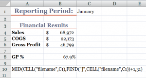
    Say, for example, that you want Cell C1 to contain the name of the current worksheet (Sheet1). With this formula, when you change the name of the worksheet to “January,” cell C1 is dynamically updated to show “January.”

    Perfect for Excel Templates

    If you use a template for your monthly, regional sales or financial reports, then this Excel formula is essential. You write the formula once – using Group edit – and each worksheet in your Excel workbook will be linked to a cell in your report. Change the name of the worksheet and your report name is automatically updated.

    Functions Used in this Formula

    • CELL() – to gather information about the worksheet – in this case, the “Filename.”
    • MID() – to extract the characters in a text string – e,g, the “worksheet name.”
    • FIND() – to locate the starting point for the MID() function to extract the characters in the text.

    As the final argument for the MID() Function, I use 31 characters because that is the maximum number of characters that you can use when naming an Excel worksheet.

    Try this for yourself. Let me know how it works for you. Add your comments below.

    Download Excel Workbook for this Lesson

    Watch Video in High Definition

    Follow this link to view this video tutorial on my YouTube Channel – DannyRocksExcels
    I invite you to watch or to subscribe to my video podcast on iTunes. Follow this link to learn more about my RSS Feed.

    Share and Enjoy:
    • Add to favorites
    • Facebook
    • Twitter
    • Technorati
    • Print
    • email
    • Digg
    • StumbleUpon
    • del.icio.us
    • Yahoo! Buzz
    • Google Bookmarks
    • Orkut
    • SphereIt
    • Sphinn

    How to Use Text Functions in Excel

    Text Functions in Excel

    Text Functions

    In my experience, I find that many of my clients do not realize that Excel has many powerful – and easy to use – Text Functions.

    Even more amazing, I observe clients spending hundreds of hours and thousands of dollars “re-keying” or “manually editing” text entries that have been downloaded from a Main Frame Computer. If you – or your colleagues – have been doing this, you will want to watch this Excel Video Tutorial.

    Categories of Text Functions in Excel

    In this Excel video lesson, I demonstrate how to use three categories of Text Functions:

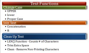
    1. Transform Text – Use the UPPER, lower and Proper functions to change the “Case” of a text string.
    2. Join Text – Use either the CONCATENATE() Function or the & (Ampersand) Operator to join two or more text strings into a single text string.
    3. Clean-up Text – Use the LEN(), TRIM() and CLEAN() Text Functions to “trim the fat” from text strings – especially those that you download from a Main Frame Computer.

    Once again, in my experience, I have too many clients contacting me in a panic because they get a REF# error when using Text Functions. I demonstrate how to recover from a “seeming disaster” and also how to use COPY – PASTE SPECIAL – VALUES to transform Formulas into Constant Values.

    I welcome your feedback. Please send me an email: danny@thecompanyrocks.com – to let me know if this tip helped you to save time and money. I also welcome your suggestions for future Excel Video Lessons to create and post here, on my website.

    Watch This Excel Video Tutorial in High Definition Mode

    Follow this link to view this Excel Video Lesson in High Defintion Mode on my YouTube Channel – DannyRocksExcels

    Download the Excel Workbook

    Follow this link to download the Excel Workbook I use in this lesson.

    Learn How to Master Excel in Minutes – Not Months!

    If you like this Excel Video Tutorial, I invite you to learn more about the resources that I offer to help you to improve your Excel skill set.

    Share and Enjoy:
    • Add to favorites
    • Facebook
    • Twitter
    • Technorati
    • Print
    • email
    • Digg
    • StumbleUpon
    • del.icio.us
    • Yahoo! Buzz
    • Google Bookmarks
    • Orkut
    • SphereIt
    • Sphinn