Refer to an Excel Table Field When Writing Formulas

Refer to Excel Table in Formula

Refer to Excel Table in Formula

While I strongly recommend creating “Named Ranges” that you can refer to in an Excel Formula, there is one drawback. By default, “named ranges” refer to “Absolute” Cells – e.g. $A$1:$A$15

However, what happens when your data set expands? For example, when you add records beyond row 15 in this case.  Now, your formulas do not refer to the additional data in each field. You need to find a way to automatically expand the range of cells that your formula refers to.

Tables in Excel 2007 and Excel 2010

Fortunately, if you are using either Excel 2007 or Excel 2010, you can “format” your data set as an EXCEL TABLE and take advantage of many great options:

  • When you append records (rows) , the definition of your Table automatically expands.
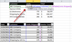
  • You can “name” your table to reflect its contents. For example, in this video I name my Table – DRTable –  and I refer to it in my formulas.

Writing Formulas that Refer to Excel Table Field

In this video tutorial I use the SUMIF Function. Remember that I have “named”my table DRTable. Here is how I begin my formula. =SUMIF(DRTable[Customer]. Notice the use of brackets ([ ]) around the [Customer] Field in the formula. This is the gotcha step in this lesson.

Watch This Video in High Definition on YouTube

I created this video tutorial in High Definition Mode. Click on this link to view it on my YouTube Channel – DannyRocksExcels

Get my best-selling DVD-ROM, “The 50 Best Tips for Excel 2007” – Visit my Online Bookstore for more information.
Share and Enjoy:
  • Add to favorites
  • Facebook
  • Twitter
  • Technorati
  • Print
  • email
  • Digg
  • StumbleUpon
  • del.icio.us
  • Yahoo! Buzz
  • Google Bookmarks
  • Orkut
  • SphereIt
  • Sphinn

How to Maintain Accurate Subtotals When Your Data Set Expands in Size

Subtotal in Excel 2010 Table

Subtotal in Excel 2010 Table

This is Part 2 of my series of video tutorials demonstrating how to use the SUBTOTAL Function in Excel.

  • In Part 1, I showed you the value of using the Subtotal Function to summarize the results of applying a Data Filter to a range of cells.
  • In this part, I show you how to use an Excel 2007 or Excel 2010 Table to ensure that your Subtotal Formulas are automatically updated when you append records or add additional fields to your original data set.

I strongly recommend basing Filtered Lists and Pivot Tables on an Excel Table (in Excel 2007 or 2010) or an Excel List in Excel 2003. This way, any formulas, filters and references that you make will be automatically updated when you append additional records or otherwise change the structure of your data set.

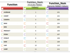
Function Numbers 101 through 111

Notice that when you “toggle on” the Total Row for a Table or List that Excel uses this formula = SUBTOTAL(109, Table1, [Sales]). Function 109 will use the SUM Function(109) to total the values in the “Sales” field ([Sales]) of a Table named “Table1.” These Function Numbers + 100 were introduced in Excel 2003 and the are automatically applied whenever you are using a Total Row in an Excel Table.

I think that you will learn some cool tricks in this lesson. Let me know what you think!

Watch This Video in High Definition

Click on this link to watch this video tutorial in High Definition, Full Screen Mode on my YouTube Channel – DannyRocksExcels.

Invitation to Visit My New Online Shopping Site

I invite you to visit my new, secure online shopping website – http://shop.thecompanyrocks.com

Once there, you can get my best-selling DVD-ROM, “The 50 Best Tips for Excel 2007”

Share and Enjoy:
  • Add to favorites
  • Facebook
  • Twitter
  • Technorati
  • Print
  • email
  • Digg
  • StumbleUpon
  • del.icio.us
  • Yahoo! Buzz
  • Google Bookmarks
  • Orkut
  • SphereIt
  • Sphinn

Don’t Subtotal Excel Data, Use Subtotal Function Instead

Subtotal Function

Subtotal Function Numbers

I used to love creating Subtotaled Reports. They are useful. They are easy to create. But they are also “clunky.” In my opinion, there are too many steps to take when you wish to see a Subtotal for a different field or to use a different function in your Subtotals.

Let me introduce you to the Subtotal Function in Excel. Here are several ways to take advantage of this function:

  • You can place the Subtotal Function in any cell on your worksheet – it does not have to reside directly below your data field.
  • You can use the Subtotal Function in connection with Data Filters – to get the subtotal for the visible cells in a filter.
  • You can use any of the 11 functions available to the Subtotal Function (Sum, Average, Count, etc.)

Watch This Video in High Definition on YouTube

This file size for this video is a little bigger than usual. So, to watch it, click on this link to view it in High Definition Mode on YouTube.

Subtotal Function Part Two

I have decided to film a second video lesson on the topic of the Subtotal Function – Using Subtotal Function in Excel Tables and Lists. Click on this link to watch my second video on this topic.

Watch or Download My 24 minute Introduction to Pivot Tables Video Recording

I have started to posted a series of “extended length” video tutorials online at: http://thecompanyrocks.webex.com – Follow this link to get more information about viewing or downloading my “free” Introduction to Pivot Tables.”

Get my best-selling DVD-ROM, “The 50 Best Tips for Excel 2007” for only $29.97!

Share and Enjoy:
  • Add to favorites
  • Facebook
  • Twitter
  • Technorati
  • Print
  • email
  • Digg
  • StumbleUpon
  • del.icio.us
  • Yahoo! Buzz
  • Google Bookmarks
  • Orkut
  • SphereIt
  • Sphinn

How to Sort Using a Custom List in Excel

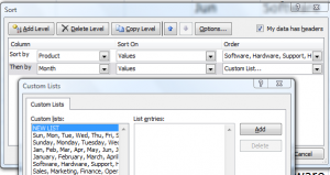
What happens when you sort a list of Months in the Year in Ascending Order? You will get “April, August …, etc.” And that, I guarantee, is not what you want! So, how do you get the list to sort as “Jan, Feb, Mar, … etc.?

Sort Using a Custom List

Sort on Custom List

Sort on Custom List

The months of the year and the days of the week are Custom Lists that are built into Excel by default. You can also create your own Custom Lists – e.g. a list of department in the order that you want to see them displayed. Once you have a Custom List saved in Excel, you can choose to sort using this order.

Watch this short video lesson to see how to create a Custom List and also how to Sort Using a Custom List in Excel.

High Definition, Full Screen Mode on YouTube

Here is the link to watch this video on my YouTube Channel – DannyRocksExcels

Learn More About Custom Lists in Excel

I have identified “Creating Custom Lists to AutoFill and Sort By” as an Essential Skill in Excel. I have created a four-hour comprehensive video training package that covers the “Nine Essential Skills in Excel.”  Click on these links to learn more about my video training resources:

Share and Enjoy:
  • Add to favorites
  • Facebook
  • Twitter
  • Technorati
  • Print
  • email
  • Digg
  • StumbleUpon
  • del.icio.us
  • Yahoo! Buzz
  • Google Bookmarks
  • Orkut
  • SphereIt
  • Sphinn

I Picked Up a New Tip Today – Filtering Your Excel Data

Yesterday, I posted an Excel Video Lesson on how to Filter your data. I focused on taking advantage of the Date Filters, Text Filters, and Number Filters introduced in Excel 2007. Today, in my email inbox, I received a great tip from Chandoo – whose tag line is “Become Awesome in Excel.”

Chandoo’s Tip – which I did not know – is to Right Mouse Click on any cell in your Excel Data Set and choose Filter – Filter by Selected Cell’s Value. As Chandoo points out, this only works in Excel 2007 and higher versions. I already use this tip in Microsoft Acces. In fact it is one of the Video Tips that I share on my DVD-ROM, “The 50 Best Tips for Access 2007.” So why didn’t I know that this would work the same way in Excel 2007? Because, I needed someone to point this out to me. Thank you Chandoo!

For me, the take-away point is to continue to explore other resources to learn from other expert users. Each – e.g. Mr. Excel – Bill Jelen; Mr. Spreadsheet – John Walkenbach, etc.) – has their own perspective on Excel. Each presents a topic in a slightly different manner. Each day is an opportunity to expand my knowledge base.

I also picked up another tip from Chandoo’s post – use the Ctrl + Shift + L Keyboard Shortcut to automatically add the Filter Drop Down Buttons to your Field Header Labels. I will use this tip on a regular basis. Now, I do not have to pick up the mouse to go to the Data Tab on the Ribbon and select Filter.

If you are using Excel 2007 and higher, note that you can also use this tip (rightmouse click in a cell) to filter by the selected cell’s Icon, Font Color and Cell Background Color. Data Visualization is one of the really great improvements introduced in Excel 2007. Click here to go to my video lesson on Data Visualization.

Tip from Chandoo
Chandoo’s Tip

I recommend that you check out Chandoo’s Excel Blog by clicking on this link. You can click on the RSS Button – or go to http://feeds2.feedburner.com/PointyHairedDilbert directly to start receiving Chandoo’s Excel tips delivered automatically to your e-mail Inbox.

 
And, by the way, you can receive my new posts automatically by going to http://feeds.feedburner.com/DannyRocks which is my RSS feed on Feedburner.
 
I have now added Chandoo’s site to my Blogroll – so just click on the link whenever you visit The Company Rocks website.
 
Let me know if you have a special tip or a favorite website or blog that you want to share with our readers. Add your comment below.
Share and Enjoy:
  • Add to favorites
  • Facebook
  • Twitter
  • Technorati
  • Print
  • email
  • Digg
  • StumbleUpon
  • del.icio.us
  • Yahoo! Buzz
  • Google Bookmarks
  • Orkut
  • SphereIt
  • Sphinn

My Most Viewed and Downloaded Videos for Excel and PowerPoint

My iTunes Podcast

Danny on iTunes

I began to post my videos as podcasts at the iTunes store this past summer. Since then, my video lessons for Excel and PowerPoint have been viewed and downloaded many times. I am thirlled. And, I thank you for your support and encouragement.

Here are the links – on my website – to the most popular video episodes. I have organized them by category in the order of their popularity. You can click on any link to view or download that video from my website. Or, you can go to my video Podcast by clicking on this link – “Danny Rocks Tips and Timesavers” Podcast on iTunes.

Merging and Consolidating Excel Worksheets

 PowerPoint Presentations

Data Visualizations

What-If Analysis in Excel

Importing Data From Other Programs

Pivot Tables

Excel Tables

Social Media

Formula Errors

Please add your comments below – or on my iTunes Channel. I welcome your feedback.

You can learn how to “Master Excel in Minutes – Not Months!”

Sincerely,

Danny Rocks

Share and Enjoy:
  • Add to favorites
  • Facebook
  • Twitter
  • Technorati
  • Print
  • email
  • Digg
  • StumbleUpon
  • del.icio.us
  • Yahoo! Buzz
  • Google Bookmarks
  • Orkut
  • SphereIt
  • Sphinn

Use an Excel Data Table to See Effect on Multiple Formulas

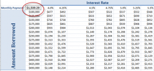
Excel Data Tables are part of the “What-if” Analysis group of tools and commands. In this lesson, I demonstrate how to use a one-input Data Table to show how substituting a series of inputs effects three separate formulas. This is a powerful – and easy – way to get answers to a series of “What-if” questions.

Data Table

2-Input Data Table

Two-Input Data Table

I know that as I learned how to construct Data Tables, it was a lot easier for me to “see” how to set them up rather than to “read about” how they are set up. You can put your series of substitute values in either the “Column running down” or the “row going across” in the data table. To include the three formulas in the Data Table, I simply included “Links” to the formulas in the original assumptions table.

Learn More About “What-if Analysis Tools in Excel

I have identified “What-if” Analysis as one of my “Nine Essential Skills for Excel.” You can learn more about my 4 hour video tutorial package by clicking on either of these links:


Share and Enjoy:
  • Add to favorites
  • Facebook
  • Twitter
  • Technorati
  • Print
  • email
  • Digg
  • StumbleUpon
  • del.icio.us
  • Yahoo! Buzz
  • Google Bookmarks
  • Orkut
  • SphereIt
  • Sphinn

Quickly Fill In all Blank Cells in Excel Report

Frequently clients will show me a report that they have downloaded from a Main Frame Computer or a Database Report. The report contains multiple blank cells. In order for my client to insert a Pivot Table or to perform Subtotals, they must fill in the blank cells by copying the value for the cell above. I have watched, in amazement, as clients copy and paste – or even type in – the missing values. There is an efficient way to perform this task. Here are the Excel Concepts that I cover in this short – 3 minute – Excel video training lesson:

  • Go To Special – Current Range
  • Go To Special – Blank Cells
  • Use Ctrl + Enter to register the formula into each cell in the selected range
  • Copy, Paste Special Values to convert formulas to values

This tip will save you lots and lots of time and prevent careless data entries. If you like this tip, I have 50 similar tips to offer you on my DVD, “The 50 Best Tips for Excel 2007.” Click here to add my DVD to your Shopping Cart.

Learn how you can “Master Excel in Minutes – Not Months!”

Share and Enjoy:
  • Add to favorites
  • Facebook
  • Twitter
  • Technorati
  • Print
  • email
  • Digg
  • StumbleUpon
  • del.icio.us
  • Yahoo! Buzz
  • Google Bookmarks
  • Orkut
  • SphereIt
  • Sphinn

Dynamically Expand the Source Data for Pivot Tables in Excel 2007

Without question, the new Tables Tools is my favorite feature  in Excel 2007 – this feature, alone, is worth the price to upgrade!

When you format a Data Range as a Table in Excel 2007, you can “append” new data to the table and the Table definition automatically expands to incorporate the new cells! If you create Pivot Tables based on a “Named Range” for your source data, this is GREAT NEWS!

Now, after appending the new data to your “Named Table: in Excel 2007, when you refresh your Pivot Table, you automatically get updated data in your Pivot Table report.

This can save you hours each month – at what – $50.00 per hour? $100.00 per hour? Watch these savings add up each month of the year

(Note: This is a re-post so that I can feed this video to my Podcast at the iTunes store.)

Follow this link, to view and download – for free – the episodes on my Podcast, “Danny Rocks Tips and Timesavers” at the iTunes store.

Learn how to “Quickly Create Excel Pivot Tables and Charts.”

Share and Enjoy:
  • Add to favorites
  • Facebook
  • Twitter
  • Technorati
  • Print
  • email
  • Digg
  • StumbleUpon
  • del.icio.us
  • Yahoo! Buzz
  • Google Bookmarks
  • Orkut
  • SphereIt
  • Sphinn

Five Benefits from Using Tables in Excel 2007

I really enjoy the major changes that Excel 2007 has incorporated into Tables. In this video I demonstrate Five Benefits when you convert your Excel data lists into Tables.

(Note: This is a re-post. I now make many of my videos available as Podcasts and I need to send these videos to the iTunes store.)

Click here if you would like to subscribe to my Podcast at the iTunes store.

Learn how to “Master Excel in Minutes – Not Months!”

Share and Enjoy:
  • Add to favorites
  • Facebook
  • Twitter
  • Technorati
  • Print
  • email
  • Digg
  • StumbleUpon
  • del.icio.us
  • Yahoo! Buzz
  • Google Bookmarks
  • Orkut
  • SphereIt
  • Sphinn