Write an Excel Macro in VBA to Update Worksheet Tab Name

Characters Not Allowed in Worksheet Names

Characters Not Allowed in Worksheet Names

This is Part 2 of my two-part series of video tutorials where I demonstrate how to link an Excel Worksheet Tab Name and the contents of a Worksheet Cell.

In this lesson, I show you how to write an Excel Macro in VBA (Visual Basic for Applications) that will update the name of the Worksheet Tab based on the value of a cell in that worksheet.

Write Excel Macro in VBA

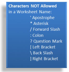
For this Macro, the first line of code will prevent the Macro from crashing if the cell contains one of the “disallowed” characters that you see in the diagram

On Error Resume Next

The second line of code initiates a “For – Next” loop of instruction

For Each ws In Thisworkbook.Worksheets

The third line of code is the Instruction to follow in the “For – Next” Loop

ws.Name = Left(ws.Cells(1,5).Value, 31)

Here, this instruction is saying – in plain English – “Nane this Worksheet (ws) using the leftmost 31 characters in the cell that is in the 1st row of the 5th column – (Cell E1)”

The reason for including 31, is that that is the maximum number of characters allowed in an Excel Worksheet Tab Name.

The fourth and fifth lines of code complete the macro – watch the video to see what they are (What a “tease” I am!!)

Run Macro from Command Button

In this lesson I also show you how to run this Macro from a command button that I add to the Quick Access Toolbar in Excel 2007 or Excel 2010.

Watch Video in High Definition on YouTube

 Click on this link to watch this Excel Video Tutorial in High Definition on my YouTube Channel – DannyRocksExcels

Source for This Code

I found the code for this example in one of Bill Jelen, Mr. Excel’s Books, “Excel Gurus Gone Wild.”

Bill’s website is: http://www.mrexcel.com/

Watch Part 1 of this Series

Here is the link to Part 1 of this series. I show you how to write a Custom Excel Function to insert the Name of the Worksheet Tab into a cell on the worksheet.
Share and Enjoy:
  • Add to favorites
  • Facebook
  • Twitter
  • Technorati
  • Print
  • email
  • Digg
  • StumbleUpon
  • del.icio.us
  • Yahoo! Buzz
  • Google Bookmarks
  • Orkut
  • SphereIt
  • Sphinn

Write a Custom Excel Function to Link Worksheet Tab Name to a Cell

Custom Functions in Excel

Custom Excel Functions

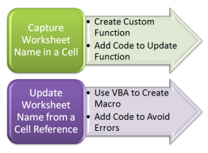
In response to many viewer requests, I am creating a two-part series of video tutorials that show you how to create links between the name of an Excel Worksheet Tab and a cell on that worksheet.

Here, in Part One, I demonstrate how to write a Custom Excel Function to capture the name of the worksheet tab in a cell.

Write Custom Excel Functions

You write Custom Excel Functions in the Visual Basic Editor. One way to open the Visual Basic Editor is to use the keyboard shortcut Alt + F11. Here are the elements that I use in this lesson:

  • Open the Project Explorer Pane (Keyboard Shortcut Ctrl + R).
  • Insert a Module to contain the VBA Code that you write for your Custom Function
  • Open the Code Pane (Keyboard Shortcut F7).

Write the Code for the Custom Function

In its simplest form, this is all of the code that you need for this Custom Excel Function:

Function SHEETNAME2() As String
SHEETNAME2 = Application.Caller. Parent.Name
End Function


That’s it!

Automatically Update Results of Custom Functions

A major difference between Custom Functions that you write and Excel’s Built-in Functions is that by default, the result of a Custom Function does not automatically update when values or references change. If you want your Custom Function to automatically update whenever the worksheet changes, add this line of code to your Custom Function in the Module:

Application.Volatile True

Source for this Code

I found the code for this Custom Excel Function in John Walkenbach’s Book, “Excel 2007 Formulas. He is an Excel Expert and I admire his writing style. You can check out his reources at this site:

http://spreadsheetpage.com/

Watch this Video in High Definition on YouTube

Click on this link to view this Excel Tutorial on my YouTube Channel – DannyRocksExcels.

Watch Part 2 of This Series

Here is the link to Part 2 in this Series. In this lesson I show you how to write an Excel Macro in VBA to update the Name of the Worksheet Tab based upon the value in a cell on the worksheet.

Share and Enjoy:
  • Add to favorites
  • Facebook
  • Twitter
  • Technorati
  • Print
  • email
  • Digg
  • StumbleUpon
  • del.icio.us
  • Yahoo! Buzz
  • Google Bookmarks
  • Orkut
  • SphereIt
  • Sphinn

How to Use an Excel Macro to Quickly Fill in Blank Cell Labels

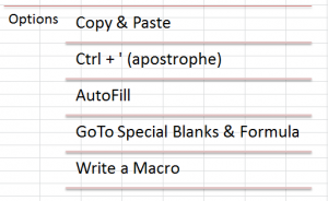
Options for Filling in Blank Cell Labels

Options for Filling in Blank Cell Labels

In this Excel video tutorial, I demonstrate how to write, proofreed and run a Macro that will quickly fill in values for blank cell lables in a report that you may have received from a colleague or a client.

Reports With “Holes in the Data”

Frequently, when you receive a report that was created in an Excel Pivot Table or from a relational database – e.g. MS Access – the report looks great! However, if you wish to apply filters or other analysis to this report, you will need to fill in the “missing” or blank cell labels.  

Watch This Excel Video Tutorial in High Definition

Follow this link to view this lesson in High Definition, Full Screen Mode on my YouTube Channel – DannyRocksExcels

Related Excel Video Tutorials

If you would like to learn how to convert an Excel Pivot Table to a Standard List – and to Fill in the Blank Cell Labels – click on this link to see my video tutorial on this topic.

And, here is a link to another related Excel Video Tutorial – Quickly Fill in Blank Cell Labels

Share and Enjoy:
  • Add to favorites
  • Facebook
  • Twitter
  • Technorati
  • Print
  • email
  • Digg
  • StumbleUpon
  • del.icio.us
  • Yahoo! Buzz
  • Google Bookmarks
  • Orkut
  • SphereIt
  • Sphinn

How to Take Advantage of Excel 2007 – 2010 Tables and Excel 2003 Lists

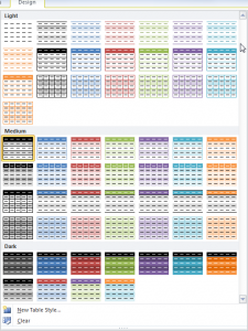
Excel Table Styles

Excel Table Styles

In this video tutorial, I cover multiple versions of Excel. I demonstrate how to take advantage of the Table Tools that were introduced in Excel 2007 and I also show you how to create Excel 2003 Lists.

Topics Covered on Video Tutorial

  • Convert a range of data to an Excel 2007, Excel 2010 Table.
  • Convert a range of data to an Excel 2003 List.
  • View and change the Total Row in each version of Excel.
  • Append new records to Tables and Lists.
  • Add a new field to Tables and Lists.
  • Write a formula in one cell of an Excel Table and have it automatically copy down for each record.
  • Change the Table Styles in Excel 2007 and 2010.
  • Use Conditional Formatting to add alternate row shading to an Excel 2003 List

Watch Video in High Definition on YouTube

Follow this link to watch this Excel Video Tutorial in High Definition on my YouTube Channel, DannyRocksExcels

Download This Excel Workbook

Click on this link to download the Excel Workbook that I used in this video tutorial.

Get my best-selling DVD-ROM, “The 50 Best Tips for Excel 2007” for only $39.95!

Share and Enjoy:
  • Add to favorites
  • Facebook
  • Twitter
  • Technorati
  • Print
  • email
  • Digg
  • StumbleUpon
  • del.icio.us
  • Yahoo! Buzz
  • Google Bookmarks
  • Orkut
  • SphereIt
  • Sphinn

Refer to an Excel Table Field When Writing Formulas

Refer to Excel Table in Formula

Refer to Excel Table in Formula

While I strongly recommend creating “Named Ranges” that you can refer to in an Excel Formula, there is one drawback. By default, “named ranges” refer to “Absolute” Cells – e.g. $A$1:$A$15

However, what happens when your data set expands? For example, when you add records beyond row 15 in this case.  Now, your formulas do not refer to the additional data in each field. You need to find a way to automatically expand the range of cells that your formula refers to.

Tables in Excel 2007 and Excel 2010

Fortunately, if you are using either Excel 2007 or Excel 2010, you can “format” your data set as an EXCEL TABLE and take advantage of many great options:

  • When you append records (rows) , the definition of your Table automatically expands.
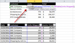
  • You can “name” your table to reflect its contents. For example, in this video I name my Table – DRTable –  and I refer to it in my formulas.

Writing Formulas that Refer to Excel Table Field

In this video tutorial I use the SUMIF Function. Remember that I have “named”my table DRTable. Here is how I begin my formula. =SUMIF(DRTable[Customer]. Notice the use of brackets ([ ]) around the [Customer] Field in the formula. This is the gotcha step in this lesson.

Watch This Video in High Definition on YouTube

I created this video tutorial in High Definition Mode. Click on this link to view it on my YouTube Channel – DannyRocksExcels

Get my best-selling DVD-ROM, “The 50 Best Tips for Excel 2007” – Visit my Online Bookstore for more information.

Share and Enjoy:
  • Add to favorites
  • Facebook
  • Twitter
  • Technorati
  • Print
  • email
  • Digg
  • StumbleUpon
  • del.icio.us
  • Yahoo! Buzz
  • Google Bookmarks
  • Orkut
  • SphereIt
  • Sphinn

How to Maintain Accurate Subtotals When Your Data Set Expands in Size

Subtotal in Excel 2010 Table

Subtotal in Excel 2010 Table

This is Part 2 of my series of video tutorials demonstrating how to use the SUBTOTAL Function in Excel.

  • In Part 1, I showed you the value of using the Subtotal Function to summarize the results of applying a Data Filter to a range of cells.
  • In this part, I show you how to use an Excel 2007 or Excel 2010 Table to ensure that your Subtotal Formulas are automatically updated when you append records or add additional fields to your original data set.

I strongly recommend basing Filtered Lists and Pivot Tables on an Excel Table (in Excel 2007 or 2010) or an Excel List in Excel 2003. This way, any formulas, filters and references that you make will be automatically updated when you append additional records or otherwise change the structure of your data set.

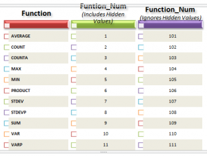
Function Numbers 101 through 111

Notice that when you “toggle on” the Total Row for a Table or List that Excel uses this formula = SUBTOTAL(109, Table1, [Sales]). Function 109 will use the SUM Function(109) to total the values in the “Sales” field ([Sales]) of a Table named “Table1.” These Function Numbers + 100 were introduced in Excel 2003 and the are automatically applied whenever you are using a Total Row in an Excel Table.

I think that you will learn some cool tricks in this lesson. Let me know what you think!

Watch This Video in High Definition

Click on this link to watch this video tutorial in High Definition, Full Screen Mode on my YouTube Channel – DannyRocksExcels.

Invitation to Visit My New Online Shopping Site

I invite you to visit my new, secure online shopping website – http://shop.thecompanyrocks.com

Once there, you can get my best-selling DVD-ROM, “The 50 Best Tips for Excel 2007”

Share and Enjoy:
  • Add to favorites
  • Facebook
  • Twitter
  • Technorati
  • Print
  • email
  • Digg
  • StumbleUpon
  • del.icio.us
  • Yahoo! Buzz
  • Google Bookmarks
  • Orkut
  • SphereIt
  • Sphinn

Don’t Subtotal Excel Data, Use Subtotal Function Instead

Subtotal Function

Subtotal Function Numbers

I used to love creating Subtotaled Reports. They are useful. They are easy to create. But they are also “clunky.” In my opinion, there are too many steps to take when you wish to see a Subtotal for a different field or to use a different function in your Subtotals.

Let me introduce you to the Subtotal Function in Excel. Here are several ways to take advantage of this function:

  • You can place the Subtotal Function in any cell on your worksheet – it does not have to reside directly below your data field.
  • You can use the Subtotal Function in connection with Data Filters – to get the subtotal for the visible cells in a filter.
  • You can use any of the 11 functions available to the Subtotal Function (Sum, Average, Count, etc.)

Watch This Video in High Definition on YouTube

This file size for this video is a little bigger than usual. So, to watch it, click on this link to view it in High Definition Mode on YouTube.

Subtotal Function Part Two

I have decided to film a second video lesson on the topic of the Subtotal Function – Using Subtotal Function in Excel Tables and Lists. Click on this link to watch my second video on this topic.

Watch or Download My 24 minute Introduction to Pivot Tables Video Recording

I have started to posted a series of “extended length” video tutorials online at: http://thecompanyrocks.webex.com – Follow this link to get more information about viewing or downloading my “free” Introduction to Pivot Tables.”

Get my best-selling DVD-ROM, “The 50 Best Tips for Excel 2007” for only $29.97!

Share and Enjoy:
  • Add to favorites
  • Facebook
  • Twitter
  • Technorati
  • Print
  • email
  • Digg
  • StumbleUpon
  • del.icio.us
  • Yahoo! Buzz
  • Google Bookmarks
  • Orkut
  • SphereIt
  • Sphinn

New Keyboard Shortcuts for Paste Special in Excel 2010

Content Key on Keyboard

Content Key on Keyboard

In Excel 2010, you can now use special keyboard shortcuts to control your Paste Special Options – e.g. Paste Values Only, Transpose, Paste Link, Paste Formatting, etc.).  There is a new technique to learn, however, before you can become proficient with these keyboard shortcuts in Excel 2010. Let me demonstrate.

Live Preview for Paste Special in Excel 2010

In my previous video tutorial, I demonstrated how to take advantage of this great new feature – “Live Preview for Pasting” – in Excel 2010. Click here to watch that video.

Two Ways to Use Keyboard Shortcuts to Paste Special in Excel 2010

  1. Press and Release the Ctrl Key, then press the “letter key” for the shortcut.
  2. Press the “Context Key” on your keyboard (to the right of the Space-bar; between the Alt & Ctrl keys) and then press the “letter key” for the shortcut.

Each of these techniques is easier to explain through a video demonstration than to write out the instructions. So, I encourage you to watch my video if you want to learn these new techniques for Excel 2010!

Learn More Paste Special Options

Main Menu Essential Skills for Excel

Main Menu for “9 Essential Excel Skills”

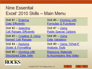
On my latest DVD-ROM, “Nine Essential Skills for Excel 2010,” I go into greater detail about the many ways that you can use Paste Special. This IS one of the 9 Essential Skills that I have identified. Follow this link to learn more about the 4 hour training video. The DVD-ROM includes 25 individual video tutorials, a 29-page instructional manual,  and the Excel 2010 Practice Files that I used while filming the videos.

Learn about all of the training resources that I offer at my secure online shopping website – http://shop.thecompanyrocks.com

Watch Video in High Definition on YouTube

Follow this link to watch this video tutorial in High Definition on my YouTube Channel – DannyRocksExcels.

Share and Enjoy:
  • Add to favorites
  • Facebook
  • Twitter
  • Technorati
  • Print
  • email
  • Digg
  • StumbleUpon
  • del.icio.us
  • Yahoo! Buzz
  • Google Bookmarks
  • Orkut
  • SphereIt
  • Sphinn

Introducing Live Preview for Paste Special in Excel 2010

Paste Special Gallery

Gallery of Paste Special Options

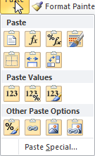
I have always loved the many “Paste Special Options” available in Excel. Now, in Excel 2010, there is a great new tool available – “Live Preview of a Gallery of Paste Special Options” – to help you to discover or to choose the best way to paste items copied to the clipboard.

From either the Paste Menu on the Home Tab of the Excel 2010 Ribbon or from the right-click shortcut menu, you can hover your mouse over one of the Gallery Icons to see a “Live Preview” of your Paste Special Option Selection.

When I demonstrate this feature  to my clients, they are amazed to discover the many options that are available! Of course, some of these same clients are also “overwhelmed” by all of the choices on the menu!

That is why I created this video – to help you to discover and to select the best Paste Special Option for your needs.

Paste Between MS Office Programs

Later in this video tutorial, I also show you how to use the Microsoft Office Clipboard and the Gallery of Paste Special Options to copy a data set from Excel and Paste it as a Picture in a Word document. With the Office Clipboard, you can cut, copy and paste up to 24 items between Excel, PowerPoint and Word. However, you must first open up the Office Clipboard for this tool to be available to use.

Additional Paste Special Features in Excel 2010

I have decided to produce an addition video tutorial to demonstrate how to use some new Keyboard Shortcuts in Excel 2010 to take advantage of the Paste Special Options.

Watch Video in High Definition Mode

Click here to watch this video in High Definition, Full Screen Mode on my YouTube Channel – DannyRocksExcels

Share and Enjoy:
  • Add to favorites
  • Facebook
  • Twitter
  • Technorati
  • Print
  • email
  • Digg
  • StumbleUpon
  • del.icio.us
  • Yahoo! Buzz
  • Google Bookmarks
  • Orkut
  • SphereIt
  • Sphinn

Two Ways to Turn Excel Data On Its Side – Transpose the Data!

Transpose Excel Data

Transpose Excel Data

How many times have you spent an hour or more creating an Excel worksheet only to discover – or be told – that you have the wrong structure? The values that you entered run vertically down in Column A. And  now, you need to have your values run horizontally across in Row 1.

Well, don’t despair! And, most important, do NOT retype your entries on another worksheet. Rather,watch this video to see how to “Turn Excel Data On Its Side”:

  1. Select Transpose from the Paste Select dialog box or the right-click shortcut menu
  2. Use the =TRANSPOSE() Function which is an Array Function

Watch as I demonstrate the advantages of each approach – they are different! If you are “curious” about how an Array Function works, the TRANSPOSE Function is a good one to practice with.

Click this link to watch this video in High Definition on YouTube.

Now Using Excel 2010

I filmed this video using Excel 2010. I will use Excel 2010 for all future video lessons unless there is a particular need to use another version to illustrate a point.

Download Workbook Used in This Video

Click on this link to download the Excel Workbook that I used in this video tutorial. It is stored on my “SkyDrive” at www.office.live.com

Get my best-selling DVD-ROM, “The 50 Best Tips for Excel 2007” for only $29.97!

Share and Enjoy:
  • Add to favorites
  • Facebook
  • Twitter
  • Technorati
  • Print
  • email
  • Digg
  • StumbleUpon
  • del.icio.us
  • Yahoo! Buzz
  • Google Bookmarks
  • Orkut
  • SphereIt
  • Sphinn