My Extended Length Pivot Tables Video Recordings Available for Excel 2003, 2007 and Excel 2010

On my WebEx site – http://thecompanyrocks.webex.com – I have posted three, one-hour-plus video recordings to help you to learn how to create and customize Excel Pivot Tables:

Download “Free of Charge” Resources for Each Recording

Click on the hyperlinks above to go to a special landing page for each Excel version. From the landing page, you will find links to download the resources that accompany each version:

  • The Excel Workbook – in each version of Excel (2003, 2007, 2010) that I use during the video recording.
  • The Step-by-Step Instructional Manual that I created for each Excel version of my recordings.
    • Available as an Adobe Acrobat PDF or as a Word Document

Very Attractive Pricing for Recordings

I have decided to price each of these recordings – which you can download to your computer – at US$9.95

  • Imagine what you would have to pay to hire a trainer – per hour –  to teach you these Pivot Table lessons!
  • Imagine how many pages in a book you would have to wade through to read about Pivot Tables!
  • Now, imagine being able to:
    • Watch a video demonstration of the steps to take to create or customize a Pivot Table.
    • Read – and make notes in – a written document that follows the steps that I demonstrate.
    • Practice the techniqes that I demonstrate on the video with the actual Excel worksheets that I use.
    • Skip back and forth to the chapter that you want to watch or review on the video recording.
    • Download the recording for the exact version of Excel that you are using.
    • Get all of this for only US$9.95

What You Will Learn on My Video Recordings

I have taken care to organize each of these topics “by chapter” – with starting points and ending points – on the recordings:

  • Create a Pivot Table in the Excel version that you are using.
    • Spotlight the uniqe features of each version
  • Filter and Sort the Fields in your Pivot Table
  • Change the Data Source & Refresh your Pivot Table
  • Use Multiple Functions and Views to Calculate your Pivot Table
  • Create a Calculated (“virtual”) Field in your Pivot Table
  • Group Fields – e.g. turn daily transactions into a Month, Quarter, Year Pivot Table Report
  • Create and Filter Pivot Charts
Download WebEx Recording

Download WebEx Recording

Download My Recordings at WebEx

  • Go to http://thecompanyrocks.webex.com and on the left side of the screen click on “Attend a Session – Recorded Sessions” to find the recording that you wish to download.
  • Register and enter your payment information – this is a secure shopping site.
  • Download the recording – also download the WebEx Recording Player so that you can play the ARF recording.
    • I recommend that you “Save” your recording on the download page. Play it from your directory of choice after it has downloaded
    • From the ARF Player for the WebEx Recording, you can convert the recording to another video format (MP4, AVI, WMV or SWF)

I welcome your feedback. Send me your questions, comments and suggestions for future recordings.

Share and Enjoy:
  • Add to favorites
  • Facebook
  • Twitter
  • Technorati
  • Print
  • email
  • Digg
  • StumbleUpon
  • del.icio.us
  • Yahoo! Buzz
  • Google Bookmarks
  • Orkut
  • SphereIt
  • Sphinn

Still Using Excel 2003? Download My Video Tutorial Pivot Tables 2003 to Summarize, Analyze and Present Data

Video Tutorial for Excel 2003 Pivot Tables

Excel 2003 PivotTables Video

By popular demand, I have created an “Extended Length” ( 69 minutes) video tutorial in Excel 2003 that you can download – for US$9.95  “Create Pivot Tables in Excel 2003 toe Summarize, Analyze and Present the Information in Your Data.”

Quite a few of my customers and viewers are still using Excel 2003. Are you one of them? If so, this is welcome news for you! If you can even find a video tutorial for Excel 2003, chances are it was created “ages ago.” I incorporate current video technology to view online or to download  69 minute video tutorial that will teach you everything that you need to know to create, modify and present a PivotTable or PivotChart Report using Excel 2003.

What You Will Learn from this Video Recording

Here are the topics that I cover – each as an individual chapter on the recording:

  • Creating a PivotTable in Excel 2003
  • Filtering and Sorting Fields in an Excel 2003 Pivot Table
  • Refreshing your PivotTable; Changing the Source Data for your Excel 2003 PivotTable
  • Changing the Functions and Type of Calculations in your Excel 2003 PivotTable
  • Creating a Calculated Field in an Excel 2003 PivotTable
  • Grouping an Excel 2003 PivotTable Field (e.g. Month, Quarter, Year from a series of Daily Transactional Data)
  • Creating and Modifying and Excel 2003 PivotChart

Skip to Individual Chapters on the Video Recording

If you have ever purchased a recording of a “live” Excel Webinar, you know that one frustration is: “How do I get to the specific part of the recording that I want to learn or repeat?”

The last thing that I want you to worry about is “getting stuck” with watching my video recording from start to finish! NO! NO! NO!

That is why I recorded this video webinar with you in mind – I created an easy to follow Table of Contents on the recording so tht you can skip to or repeat an indivual chapter or starting point!

I am confident that you will enjoy this feature!

How to Get Started

  1. Go to http://thecompanyrocks.webex.com and click on “Recorded Sessions” to see the list of all of my Recorded Video Lessons on WebEx by Cisco.
  2. Click on this link to open the Video Recording, “Excel 2003 Pivot Tables to Summarize and Analyze Data”
  3. Register for this recording (First Name, Last Name and email address) so that I can assist you quickly if you need help with downloading the recording or accessing the support materials.
  4. Enter your payment information US$9.95 using PayPal or a Credit Card – This is a SECURE WEBSITE.
  5. Download this video recording. I recommend that you: 
    1. Download the WebEx by Cisco ARF Recorder/ Player. Once you have opend the Video Recording, you can convert it to a different format (e.g. WMV (Windows Media), SWF (Flash Format) or MPEG4 (MP4 Format)
    2. Save the File to a Folder on your hard disk drive.
  6. Watch the video recording.

Download the Support Material for this Video Recording

Here is a link to the web page that I created for this video recording. Follow the hyperlinks to view online or download the Excel Workbook that I used in this recording as well as the Step-by-Step Instructional Manual that accompanies this recording.

Give Me Your Feedback

As I develop these “Extended Length” video recordings, I seek your feedback. Tell me what you liked. Tell me what you did not like – any why. Send me your suggestions for future topics for my video tutorial recordings.

Share and Enjoy:
  • Add to favorites
  • Facebook
  • Twitter
  • Technorati
  • Print
  • email
  • Digg
  • StumbleUpon
  • del.icio.us
  • Yahoo! Buzz
  • Google Bookmarks
  • Orkut
  • SphereIt
  • Sphinn

Download My 75 Minute Video Tutorial on Excel 2007 Pivot Tables

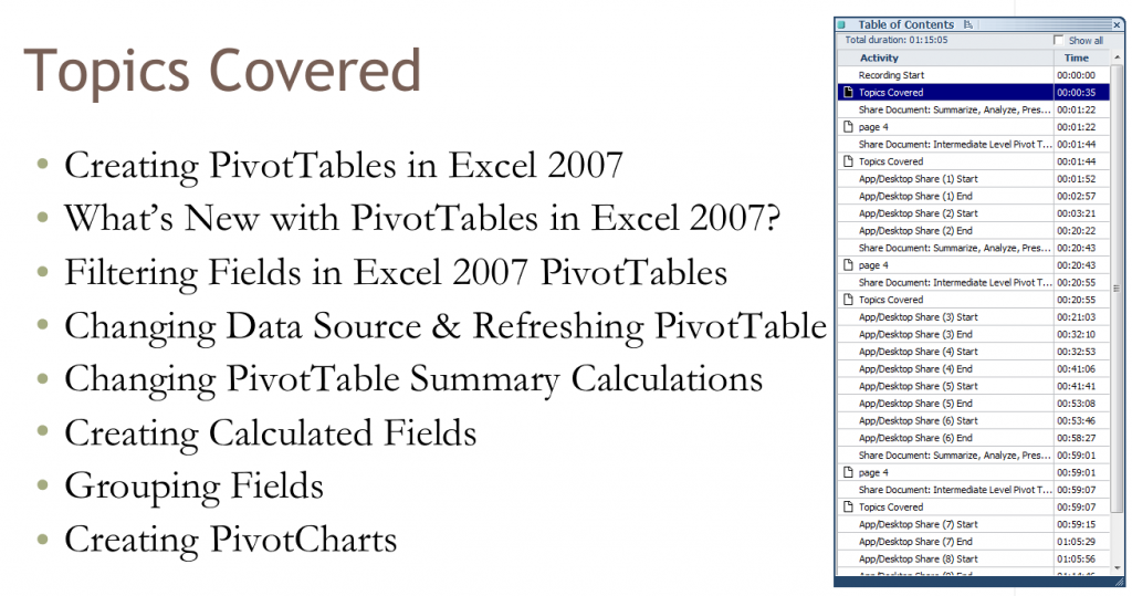
Topics Covered

Table of Contents for Recording

I have just recorded and published a 75 Minute Video Tutorial titled, “How to Create and Modify a Pivot Table in Excel 2007 to Summarize, Analyze and Present the Information in your Data Set.”

It is published on my WebEx by Cisco site: http://thecompanyrocks.webex.com Follow this link to go directly to this recording.

There is a charge for this recording – US$9.95 In addition to the recording you get:

  • A Step-by-step instructional manual
  • Access to the Excel workbook files that I used for this recording

Not to brag , but I think that this video tutorial is excellent! I spent many hours planning out the exercises, working through the timing of each chapter of the video and practicing my delivery. I am happy with the result. And, more important, I think that you will also be satisfied with what you will learn from this recording!

What You Will Learn on My Recording

My goal is to give you a comprehensive understanding of Excel 2007 Pivot Tables. But to give you the opportunity to learn this in “bite-size chunks” that can replay when necessary. I created realistic exercises to illustrate each topic.  Also notice that I have created a Table of Contents for the recording so that you can go to a specific chapter on the recording. You can stop and start at any point.

How to Download this Recording

  1. Go to http://thecompanyrocks.webex.com or click on this link to go to the main menu.
  2. Click on “Recorded Sessions.”
  3. Click the link for the recording, “Excel 2007 Pivot Tables to Summarize Data.”
  4. Register for this session (First Name, Last Name and email address).
  5. Enter payment information (PayPal or Credit Card). This is a secure site!
  6. Follow the instructions to Download my recording.
  7. Recommended – you can also download the ARF Recorder to view the recording.
  8. At this point you can decide to convert the recording to a different format. E.g. WMV (Windows Media Player), SWF (Flash) or MP4 (MPEG4)
  9. At the end of the recording, you are taken to a web page with links to download the Instructional Manual and to download the Excel Workbook that I used during this recoring.

Give Me Your Feedback

I welcome your comments and suggestions for future video tutorial recordings. You can add your comments below or send them to me via email.

Share and Enjoy:
  • Add to favorites
  • Facebook
  • Twitter
  • Technorati
  • Print
  • email
  • Digg
  • StumbleUpon
  • del.icio.us
  • Yahoo! Buzz
  • Google Bookmarks
  • Orkut
  • SphereIt
  • Sphinn

How to Apply Conditional Formatting to a Pivot Table in Excel

A Pivot Table is a great way for you to summarize and present the information contained in your data set. When you apply conditional formatting to your Pivot Table, you can “visually” spot important trends or anomolies in your data.

Improvements to Conditional Formatting

Conditional Formatting in Pivot Table

Condition Formatting for Above Average

Beginning with Excel 2007, Conditional Formatting has been dramatically improved. In addtion to pre-built formula rules, you can also apply Data Visualizations (Icon Sets, Data Bars and Color Scales).

Conditional Formatting for Above Average

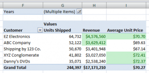
In this lesson, I apply the pre-built “Above Average” rule. I want Excel to dynamically format the summary values that answer, “TRUE” to this question: “Is this value “Above the Average” in the range of cells selected?

This is the key to understanding how Conditional Formatting works. Special Formatting is applied only when the answer to your CONDITION (a rule or a formula) is TRUE.

Dynamically Filter Conditional Formatting

In this lesson, I use the Report Filter zone in my Pivot Table to see how conditions change when I change the time period in my report. Values that meet the Condition, “Above the Average,” receive the formatting that I established in my rule. Try this on your Pivot Table. It is a wonderful tool to use in an Excel Dashboard.

View This Video Tutorial in High Definition

Follow this link to watch this lesson in High Definition on my YouTube Channel, DannyRocksExcels.

My Extended Length Pivot Table Video Tutorials

I offer “free of charge,” a 24 minute in-depth video tutorial for creating your first Pivot Table in Excel. Follow this link to learn how to view it online or to download it to your computer.

Vist My New Online Shopping Site

My new, secure online shopping website – http://shop.thecompanyrocks.com/ – is now open. I invite you to visit and learn more about the new products that I have added.

Share and Enjoy:
  • Add to favorites
  • Facebook
  • Twitter
  • Technorati
  • Print
  • email
  • Digg
  • StumbleUpon
  • del.icio.us
  • Yahoo! Buzz
  • Google Bookmarks
  • Orkut
  • SphereIt
  • Sphinn

How to Create an Interactive Pivot Chart in Excel

While I have created many Excel Video Tutorials demonstrating the power of interactive Pivot Tables during the past four years, I have NEVER created a video lesson focused on creating interactive Pivot Charts in Excel – until now!

Interactive Pivot Table Chart

Interactive Pivot Table Chart

Pivot Charts in Excel 2007

In this lesson, I show you how to create a Pivot Chart in Excel 2007. Starting with Excel 2007, there are several major changes:

  • By default, Pivot Charts are embedded on the same worksheet as the Pivot Table Report that is linked to the chart.
  • A new, PivotTable Chart Filter Dialog box is available – this works “in tandem” with the filters available in the PivotTable Field List” Dialog box.
  • It is very easy to “Move” a Pivot Chart to its own worksheet tab – or vice versa – to move the Pivot Chart to an existing worksheet.

 Pivot Charts and Pivot Table Reports are Connected

A Pivot Chart MUST be connected to a Pivot Table Report. Any changes that you make to the chart are reflected in the report and vice versa. If you filter the Pivot Table Report, the filter is automatically applied to the Pivot Chart. This is an important concept to understand. This is the reason why it is so easy to make BOTH Pivot Table Reports and Pivot Charts “interactive!”

Explore My Index of Free Excel Video Lessons

I was surprised to discover that I had not yet created a video tutorial for Excel Pivot Charts when I looked at my list of “free” Excel Video Lessons. This became the impetus for creating this lesson. I invite you to explore all of my free Excel Video Tutorials. Click on this link to go to my Index of Excel Video Lessons. I have organized the free video lessons by topic. Simply click on the title of any lesson and you will arrive at the posting and the video for that lesson.

Download Excel File for This Lesson

View this Lesson in High Definition

I invite you to view this Excel Video Tutorial in High Definition, Full-screen Mode on my YouTube Channel – DannyRocksExcel

Watch Video Now


Feedback Welcome

I always welcome your feedback. Let me know what you think about this – or any other – video lesson. Add your comments below!

Extended Length Video Training Resource for Pivot Tables

I have created 90-minutes video training resources for Pivot Tables. Follow this link to learn more about my “Master Excel in Minutes” series.

Share and Enjoy:
  • Add to favorites
  • Facebook
  • Twitter
  • Technorati
  • Print
  • email
  • Digg
  • StumbleUpon
  • del.icio.us
  • Yahoo! Buzz
  • Google Bookmarks
  • Orkut
  • SphereIt
  • Sphinn

How to Convert a Pivot Table to a Standard List

Watch this video tutorial in High Definition on YouTube

A viewer aksed for my help. She has a boss and a few customers who:

  1. Do not know how to create or use Pivot Tables
  2. Have no desire to learn how to create and use Pivot Tables
Convert Pivot Table to Standard List

Convert Pivot Table to List

Nevertheless, in this example, she is being asked to create a summary report – by Year and by Quarter – from @ 5,000 daily transaction records. The fastest way to create this report is with a Pivot Table. Now, to meet the demands of her boss and clients, she needs to convert this Pivot Table into a standard list that can be Filtered and Subtotaled.

Summarize by Year and Quarter

To create this Pivot Table report:

  • Add the “Date” field to the grid and then select a single date.
  • Group the Date field by Month, Quarter and Year.
  • Add and arrange the Customer and Invoice fields to the Pivot Table Grid.

Convert Pivot Table to Standard List

  1. Remove both the Subtotals and Grand Totals from the Pivot Table Report.
  2. In Excel 2007 & 2010, ensure that you are using either the Outline or Tabular report layouts – NOT the new “default” Compact layout.
  3. Also in Excel 2007 & 2010, remove the Field Headers and the + / – Symbols.
  4. Now, select the entire Pivot talbe (use Ctrl + A) and copy it to the clipboard.
  5. Use Paste Special Values to paste the Pivot Table Results.

Filling the Blank Cells in the List

As you can see, whenever you have “nested rows” in a Pivot Table you get a nice, clean report. However, in order to Filter and Subtotal this new list, you will need to “fill in the blank cells.”

  1. Select all of the values and all of the blanks in Column A.
  2. Use Ctrl + G (or F5) to open the Go To Dialog Box and choose Special.
  3. From the Go To Special choices choose “Blanks.”
  4. With all of the Blank Cells selected use this formula: = ↑
  5. Do NOT press Enter. Rather, press Ctrl + Enter and all of the Blank Cells are now filled in with the Customer Names!
  6. Finally use Copy, Paste Special, Values to complete this process.

Watch This Video on My YouTube Channel – DannyRocksExcels

Since this video tutorial is a little longer than usual, I have decided to post it as a video – in High Definition – on my YouTube Channel. Click here to view it or copy and paste this link into your browser:

Link to YouTube Video:   http://youtu.be/IwReVDJ7BAI?hd=1

Download This Excel Workbook

Share and Enjoy:
  • Add to favorites
  • Facebook
  • Twitter
  • Technorati
  • Print
  • email
  • Digg
  • StumbleUpon
  • del.icio.us
  • Yahoo! Buzz
  • Google Bookmarks
  • Orkut
  • SphereIt
  • Sphinn

How to Create Custom Headers and Footers for Printing Excel Worksheets

How many times have you wasted time and paper when printing out an Excel Worksheet? Did you:

  • Forget to include the page numbers in the footer of each printed page?
  • Forget to repeat the column titles for the second and succeeding pages?
  • End up with “orphaned” columns that are disconnected from the main worksheet?
Headers and Footers in Excel

Headers and Footers in Excel

And the list goes on and on and …

Most Excel users, in my experience, spend very little time “previewing” their Excel worksheet prior to printing it – and wasting time and money. And also leaving a poor professional image in the minds of their clients and colleagues. 

Don’t let this happen to you!

Page Layout View

Page Layout View is a “working” view that was introduced in Excel 2007. I spend most of this video tutorial showing you how to get the most out of Page Layout View, including the placeholders for Header and Footer Elements. Personally, I spend a considerable amount of time when I am creating a new worksheet working in Page Layout View. Here, unlike in earlier versions of Excel, you can see how adding an additional column or two will effect the printed page. You can also verify that you company logo and other elements are properly positioned – while you are working inside the worksheet! For me, this view is indispensable!

Watch Video in High Definition on YouTube

This Excel Video Tutorial is a little longer than usual – 10 minutes and 14 seconds – and it contains more graphic images than usual. So, rather than embed this as an MP4 Video, I have decided to provide the link to this video on my YouTube Channel – DannyRocksExcels. Here is the link:

 http://youtu.be/X_Pb0KNFYak?hd=1

I produced this in High Definition, Full Screen Video Mode. This video is best watched on YouTube in High Definition. Let me know what you think.

Master Excel in Minutes – Not Months!

Learn how you can quickly learn how to get the most out of Excel – in the least amount of time! Click here to find out how!

Share and Enjoy:
  • Add to favorites
  • Facebook
  • Twitter
  • Technorati
  • Print
  • email
  • Digg
  • StumbleUpon
  • del.icio.us
  • Yahoo! Buzz
  • Google Bookmarks
  • Orkut
  • SphereIt
  • Sphinn

Free Video Recording of Excel Keyboard Shortcuts to Download

I have just published a 50 Minute Video Recording on which I demonstrate the most popular Keyboard Shortcuts for Excel. The great news – for you – is that you can download this video recording for FREE! If you prefer to view this online, you can do so – for FREE!

Download My Excel Workbooks

Download my Workbooks

Download Excel Workbooks

In addition, I have published the Excel Workbooks, Adobe PDFs and PowerPoint files that I use during this 50 minute video online. You can access them – for FREE!

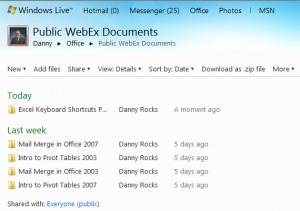
I store them as “public documents” for you to download on my “Sky Drive” at Windows Live! Here is the direct link:

http://cid-644f2f857aa6afdc.office.live.com/browse.aspx/Public%20WebEx%20Documents/Excel%20Keyboard%20Shortcuts%20Part%201

In order to access these files, you will need a “free” Windows Live account (First Name, Last Name, email address). You can also use your HotMail account to login.

My Extended Length Video Recordings on WebEx

I have recently began to publish “extended length” video recordings at http://thecompanyrocks.webex.com – This 50 Minute video is my 5th recording on the site. I offer it to you “free of charge.” However, you must register (fitst name, last name, email address) with WebEx by Cisco before you can download the recording or view the recording online.

In this format, I can offer “specialized instruction” for Excel Pivot Tables, Macros, Public Speaking Courses, etc. I can also offer instruction in older (Excel 2003) and newer (Excel 2010) programs. In addition, I can create a specialized recording “just for you.” Contact me to learn about how to organize this!

Landing Page for More Information

Links for Downloads

Information about Links and Downloads

Rather than repeat what I have already written, here is the link to the special Landing Page that I have created for this 50 minute video recording. On the Landing Page, I have included all of the direct links to the download pages for the video, the Excel files, PowerPoints and Adobe Acrobat documents that I used on this recording.

I invite you to view or download these new resources that I have made available. When you have a chance send me your comments, questions and suggestions for future recordings!

Danny Rocks

The Company Rocks

Watch This Video Lesson in High Definition

Click here to go to my DannyRocksExcels YouTube Channel where you can view this tutorial in High Definition.

Share and Enjoy:
  • Add to favorites
  • Facebook
  • Twitter
  • Technorati
  • Print
  • email
  • Digg
  • StumbleUpon
  • del.icio.us
  • Yahoo! Buzz
  • Google Bookmarks
  • Orkut
  • SphereIt
  • Sphinn

Create an Accounts Payable Summary Report in Excel

Accounts Payable Status Summary

Accounts Payable

Here is another video lesson that I created to answer a question from one of my viewers. In this case, the request is for help in creating an Accounts Payable Summary Report in Excel.

Formula to Create Label for Status

My viewer wants to know how to create one formula that will report the status of an Invoice as “Paid,” “Pay Now,” or “Delay.” To do this I “nested” one IF() formula inside another IF() formula. I used the ISBLANK() function as my first “logical test” in the formula. ISBLANK returns either TRUE or FALSE, so it is a good Function to become familiar with.

One of my “best practices” when learning how to “nest” IF Formulas, is to create each one separately – to test the results – and then copy and paste them into the combined formula.

Use SUMIF() Function to Total Status

Now, that your formula returns a status label for each invoice, you can use the SUMIF Function to search in the Named Range “Status” for the cells that match the criteria (Paid, Pay Now, Delay) and then Sum the Invoice Amounts for each category.

Watch This Video in High Definition on YouTube

Here is the link to my YouTube Channel, DannyRocksExcels, where you can watch this in High Definition.

Download this Excel Workbook

Follow this link to go to my Public SkyDrive to download this workbook to practice with.

Share and Enjoy:
  • Add to favorites
  • Facebook
  • Twitter
  • Technorati
  • Print
  • email
  • Digg
  • StumbleUpon
  • del.icio.us
  • Yahoo! Buzz
  • Google Bookmarks
  • Orkut
  • SphereIt
  • Sphinn

How to Use SUMIF in Excel to Total Year-to-Date Sales

One of my viewers asked for my help to use the SUMIF Function in Excel to total Year-to-Date (YTD) Sales. Generally, the SUMIF Function is very easy to set up and use. However, when you need to refer to a “date” in the criteria argument, there is a “Got’cha” step.

How to Write the Formula for Year-to-Date Sales

=SUMIF(Date, “<=”&TODAY(), Sales) Notice how the <= comparison operator is enclosed within ” ” (Quotation Marks) and I use the & (ampersand) to join the TODAY() Function. Be careful when you write this fomula. In my experience, when I try to write THIS formula in the “Functions Argument” Dialog Box, I almost always get an Error Message.

Create and Use Named Cell Ranges in SUMIF Function

As a best practice, I encourage you to create and use “Named Cell Ranges” in your formulas. This is especially helpful with the SUMIF, SUMIFS, COUNTIF, COUTIFS functions because you are usually looking inside extensive ranges of data.

Another Way to Total Year-to-Date Sales

For many years, I did not realize that there was a SUMIF Function. So, I used to create an extra column and write to formulas to compute the YTD Sales. If you do want to or need to see YTD sales in each cell, I show you how to do this by writing just one formula.

Watch Lesson in High Definition

Follow this link to view this video lesson in High Definition on my YouTube Channel – DannyRocksExcels

Download My Free Video Lessons on Pivot Tables

Click here to learn about my 24 minute video recordings “Introducing Pivot Tables.” I have two versions – One for Excel 2003 and one for Excel 2007. I am offering both of them as a “free of charge” downloadable product!

Share and Enjoy:
  • Add to favorites
  • Facebook
  • Twitter
  • Technorati
  • Print
  • email
  • Digg
  • StumbleUpon
  • del.icio.us
  • Yahoo! Buzz
  • Google Bookmarks
  • Orkut
  • SphereIt
  • Sphinn