How to Find and Change Numbers Stored as Text in Excel

Whenever a client or a colleague sends me an Excel workbook I like to inspect it, to be sure that the “numbers are really numbers.” I will not get accurate results when I SUM them if there are some cells that appear to contain numbers, but really display a “number stored as text.”

Prevent GIGO

Prevent GIGO

This is an example of GIGO – “Garbage in delivers Garbage Out!” I take steps to prevent an outbreak of GIGO in my Excel worksheets.

Looking for Numbers Stored as Text

As a best practice, I use both the COUNT() Function and the COUNTA() function to see if there is a difference between the number of cells with numbers (the COUNT Function) and the number of non-blank cells (the COUNTA Function). In this example, I was expecting to see 31 cells with numbers in the range of sales. There were on 27. So, I need to find those 4 cells that contain “numbers stored as text.” 

If you have a keen eye – and some time to spare – you can look for cells with a little Green triangle in the upper left corner. Click on the message next to these “marked” cells and read the error message. Excel will offer to correct the error – one cell at a time. That is not an efficient way to proceed!

Use the ISTEXT() or ISNUMBER() Functions

An alternative way to find the cells that contain text stored as numbers is to use one of the “logical functions” ISTEXT or ISNUMBER. Each returns either TRUE or FALSE when evaluating a cell. You can then sort the data to group the TRUE results together and then change them – again, one at a time. This is also not the best way to make the changes.

Use Conditional Formatting to Highlight Cells with Number Stored as Text

I like to use the ISTEXT() Function as a “Rule” to apply special formatting to the cells that evaluate as TRUE with Conditional Formatting. Be sure that you select the cells that you want to evaluate before applying the Conditional Formatting.

Use Paste Special – Add

The quickest way to change numbers stored as text into real numbers is to use Paste Special – Add. First, select and copy a blank cell. Next, select your data range – in this case the cells with “Sales.” Then, right click the selection and choose Paste Special. In the dialog box select “Add.” Now – instantly – all of the cells with numbers stored as text have been changed into real numbers. You have stamped out GIGO!

Learn how to “Master Excel in Minutes – Not Months!”

Follow this link to watch this video in High Definition, Full-screen mode on my YouTube Channel – DannyRocksExcels

Share and Enjoy:
  • Add to favorites
  • Facebook
  • Twitter
  • Technorati
  • Print
  • email
  • Digg
  • StumbleUpon
  • del.icio.us
  • Yahoo! Buzz
  • Google Bookmarks
  • Orkut
  • SphereIt
  • Sphinn

How to Find and Delete Duplicate Records in Excel 2007

It is easy  – much too easy – to allow duplicate records to creep into an Excel database. Fortunately, starting in Excel 2007, it is really easy to first find and then delete duplicate records.

Remove DUplicate Records

Remove Duplicate Records

With the price of postage climbing, you cannot afford to send duplicate copies of a mailing piece. Not to mention that doing so reflects poorly on your company’s organizational skills. Likewise, having duplicate account entries makes for extra work and confusion.

Use Conditional Formatting to Highlight Duplicate Records

Starting in Excel 2007, Conditional Formatting got a lot easier to use. One of the menu selections is “Show Duplicate Records.” Now, with just a few mouse clicks, you can format the records that show duplicate values in your data set. I like to use this technique prior to acutally duplicating records so that I can get a sense of the number of possible duplicate records in my data set.

Selecting Duplicate Records to Delete

As a best practice, I always make a backup copy of my data set before I actually delete records. This way, I can quickly recover from any accidental deletions of non-duplicate records. When you choose the command to “Remove Duplicates,” a dialog box opens to reveal each field in your data set. Generally, you want to select all of the fields to narrow down the list of records to delete. Since I have already previewed the possible duplicate records by using Conditional Formatting, I have a pretty good idea of how many records will be deleted. You do not see a preview of the exact records that will be deleted, so make sure that you have a backup copy of your original list in order to restore any “accidental” deletions.

These new commands and menus introduced in Excel 2007 make deleting duplicate records a very quick process. Use them – wisely – to save yourself time, confusion and money!

Learn how to “Master Excel in Minutes – Not Months”

Watch this video lesson in High Definition, Full Screen mode. Follow this link to view this on my YouTube Channel – DannyRocksExcels

Secure Shopping Cart

Secure Shopping Cart

This is one of the tips that I offer on my DVD, “The 50 Best Tips for Excel 2007.” CLick here to open a secure shopping cart to purchase it.

Share and Enjoy:
  • Add to favorites
  • Facebook
  • Twitter
  • Technorati
  • Print
  • email
  • Digg
  • StumbleUpon
  • del.icio.us
  • Yahoo! Buzz
  • Google Bookmarks
  • Orkut
  • SphereIt
  • Sphinn

How to Convert from Military to Standard Time in Excel

Viewers and clients frequently ask me how to convert times displayed as military time (1700 hours) to standard time (5:00 PM). Many conpanies capture time using the 24 hour clock (military time) however, many end-users, particularly in the United States want to see time expressed as standard time with AM and PM designations. 

Time on Clock

Digital Time

Time Stored as Text Value or as a Number?

The first step in the conversion is to determine how the time value is “stored” in Excel. Is it stored as a “text value” or is it stored as a numeric value? This will determine how we convert military time to standard time. In this lesson, I demonstrate how to extract text characters, join text strings and then use the TIMEVALUE() Function in Excel to make this conversion. 

Use Text Functions and the “&” (ampersand)

Next, I use the LEFT() function to extract the two left-most characters from the text string (0100) and the RIGHT() function to extract the two right-most characters. In Excel, you use the “&” (ampersand) to join text strings. When you insert the “:” (colon) between the hours and the minutes, be sure to enclose it inside ” “(double quote marks). 

The TIMEVALUE() Function

In order to perform time elapsed calculations in Excel, you need to have time values “stored” as numeric values. You can use the “visual clue” – to which side of the cell is the time value aligned? Text values align to the left side of the cell; numeric values align to the right side of the cell. After you use the TIMEVALUE() function, be sure to format the numeric time values to meet your needs. 

If you import time values that are “stored” as numbers – they align to the right side of the cell – but are formatted as military time (13:30) all you have to do is change the fomratting to standard time (1:30 PM). 

Follow this link to watch this video lesson in High Definition, Full Screen mode on YouTube. My channel is DannyRocksExcels.

I invite you to subscribe to my video podcast, “Danny Rocks Tips and Timesavers,” available for free on iTunes. Click here to view my videos at the iTunes store.

Visit My New Online Shopping Website

I invite you to visit my new, secure shopping website – http://shop.thecompanyrocks.com – where you can view all of my products and “Learn how to “Master Excel in Minutes – Not Months!”

Share and Enjoy:
  • Add to favorites
  • Facebook
  • Twitter
  • Technorati
  • Print
  • email
  • Digg
  • StumbleUpon
  • del.icio.us
  • Yahoo! Buzz
  • Google Bookmarks
  • Orkut
  • SphereIt
  • Sphinn

Working With Array Formulas in Excel

There are at least two benefits to using an Array Formula in Excel:

  1. They will speed up creating your formulas by, in many cases, eliminating intermediate formulas.
  2. They will add a level of protection to your formulas because you cannot edit the individual cells in an Array Formula. You must edit “all” of the cells.
Array Formulas
Array Formulas

In this lesson, I first demonstrate how to select and use arrays with the SUMPRODUCT() Function in Excel. SUMPRODUCT is a very handy function to use when you want to first multiply (PRODUCT) the cells in two or more arrays and then total (SUM) the results.

 
Next, I demonstrate two ways to create Array Formulas. Notice that in the second example that it is important that you remember to select ALL of the cells that will contain the results of the Array Formula. It is vital that all arrays are of Equal Size (Same number of cells in the same dimension – horizontal and vertical).
 

Entering Array Formulas

Use the keyboard combination of Ctrl + Shift + Enter when entering an Array Formula. Do not press the Enter key alone – this will result in an Error for your formula! Some people refer to Array Formulas as CSE Formulas to remember the Ctrl + Shift + Enter combination. Notice, in the Formula Bar,  that Excel automatically adds { braces } around the Array Formula. Do not enter these manually.

Editing Array Formulas

You gain a level of protection for your formulas when you use Array Formulas because you cannot select a single formula cell to edit it. You must select all of the cells that contain the Array Formula before you can edit it – or delete it. If you don’t select all of the cells first, you receive an Error message in a pop-up window. Remember to press the “CSE keyboard combination” when you complete your edit of the Array Formula.

Learning to use Array Formulas is an essential skill to acquire if you want to master Excel. I guarantee that you will be able to write more accurate formulas when you use arrays.

Watch this Video on YouTube

Click this link to watch this Excel Video in High Definition, Full Screen Mode on my YouTube Channel – DannyRocksExcels

Learn how to “Master Excel in Minutes – Not Months!”

Share and Enjoy:
  • Add to favorites
  • Facebook
  • Twitter
  • Technorati
  • Print
  • email
  • Digg
  • StumbleUpon
  • del.icio.us
  • Yahoo! Buzz
  • Google Bookmarks
  • Orkut
  • SphereIt
  • Sphinn

How to Use Date Functions and Date Formatting in Excel

In this lesson, I respond to two recent requests from viewers for help in Using DATE Functions in Excel and also, how to apply Custom Date Formatting. I get similar requests on a frequent basis from both viewers and clients.

Solve Problem #1 

My first viewer wants help in using the DATE() Function in Excel. She wants to calculate a date that is 90 days after the starting date for a project. She encountered two problems

  1. Initially, the DATE() Function produced and error – because she forgot to ‘nest” the YEAR(), MONTH()+9, DAY() Functions inside the DATE() Function.
  2. She was not expecting a date to be filled in the formulas column when there was no starting date for the project – She needed to include an IF() function to perform a LOGICAL TEST – Does  the Starting Date = 0, Value if TURE, ” ” (to display nothing), Value if FALSE – to perform the calculation.
Excel Custom Date Formats

Excel Custom Date Formats

Solve Problem #2

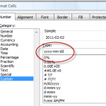
My second viewer wanted my help to ensure that the date values that he “pasted” into a range of cells were in the (Custom) format of “yyyy-mm-dd” (Year, Month, Date).

In this case, we need to take two steps:

  1. Format the destination cells using the CUSTOM FORMAT of yyyy-mm-dd that we create.
  2. After “Pasting” the Copied Cells, use the “Paste Options” dialog box to select – “Match Destination Formatting.”

I also demonstrate how to use the NETWORKDAYS() Function and the WORKDAY() Function – with an optional list of “Holidays” to exclude. And, finally, I show you the “pitfalls” that occur when you import a “text” file of dates that use a variety of formats. In order to perform DATE calculations, a date must be stored as a NUMBER in Excel. It must be right-aligned in the cell.

You can watch this Excel Video Lesson in High Definition, Full Screen Mode on my YouTube Channel – DannyRocksExcel – by clicking this link.

Learn to “Master Excel in Minutes – Not Months!”

Share and Enjoy:
  • Add to favorites
  • Facebook
  • Twitter
  • Technorati
  • Print
  • email
  • Digg
  • StumbleUpon
  • del.icio.us
  • Yahoo! Buzz
  • Google Bookmarks
  • Orkut
  • SphereIt
  • Sphinn

How to Use Conditional Formatting to Compare Two Excel Lists

Clients and viewers frequently ask me to help them to compare two differeny lists in Excel. They want to find – or highlight – the values that are different in each list. For example, which customers appear in the 1st list but NOT in the 2nd list. So, I created this video lesson to demonstrate how to do this with Conditional Formatting.

In an earlier Excel Video Lesson, I demonstrated how to compare two Excel lists using either the MATCH() Function or the VLOOKUP() Function.

Conditional Formatting Rule

Conditional Formatting Rule

Use Conditional Formatting

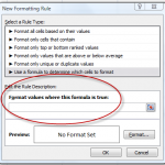
I demonstrate how to use Conditional Formatting to Highlight the Cell Values that are different when you compare two Excel Lists. I will use a “New Rule with a Formula” that must return the answer TRUE, to trigger the special formatting.

In Conditional Formatting, you first establish a “condition” that can be answered as either TRUE or FALSE. Then, for those cells where the answer to the condition is TRUE. the special “cell formatting” that you chose will apply.

In this lesson we will be using this Formula: =COUNTIF(List 2, 1st cell in List 1) = 0.

Steps to follow:

  1. Select the cells that you want the Conditional Formatting to apply to- in our example List 1.
  2. On the Home Tab of the Ribbon, click the Conditional Formatting arrow and select New Rule.
  3. Select New Rule – “Use a Formula to determine which cells to format.”
  4. Enter the formula – e.g. =COUNTIF(Range, Criteria) = 0 where the “Range” is the list of values in List 2 (Absolute Reference) and the “Criteria” is the 1st cell reference in List 1 (Relative Reference).
  5. Choose the Format for the cells when the condition is met – the result is TRUE. In this example, I choose to “FILL” the cells with a Blue background color.

Want to watch this video in High Definition, Full-Screen Mode? Click here to go to my YouTube Channel, DannyRocksExcels

Learn to “Master Excel in Minutes – Not Months!”

Share and Enjoy:
  • Add to favorites
  • Facebook
  • Twitter
  • Technorati
  • Print
  • email
  • Digg
  • StumbleUpon
  • del.icio.us
  • Yahoo! Buzz
  • Google Bookmarks
  • Orkut
  • SphereIt
  • Sphinn

How to Calculate Overtime and Standard Hours Worked on a Time Card in Excel

One of my viewers asked me to show him how to calculate the number of hours worked each day – separated by standard hours and by overtime hours. He, like many Excel users, is frustrated when performing calculations involving time. They create a standard formula, but the results are not what they were expecting. In most cases, this is because of the need to FORMAT the cells that contain calculations to accommodate Excel’s logic.

Excel Time Card

Excel Time Card

Time Functions and Formats

In this lesson, I demonstrate the following functions and formats:

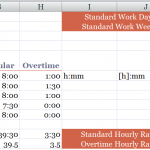
  • The =TIME() Function requires three arguments (Hours, Minutes, Seconds). In this example, I use =TIME(8,0,0) in a cell to represent the Standard Hours Worked each day – i.e. 8 hours.
  • The CUSTOM Format h:mm to format the cells that contain the results of time calculations (Total Hours Worked each day, Regular and Overtime Hours Worked each day).
  • The CUSTOM Format [h]:mm to format the cells that contain the results of SUM() for the Total Hours, Regular and Overtime Hours Worked each WEEK – i.e. Hours that exceed 24 hours
  • The Formula =SUM(Overtime Hours Worked this week) * 24 to gives me the NUMBER equivalent – Remember to format this cell as a NUMBER – not as [h]:mm,  so that you can multiply it by the cell that contains the Hourly Rate that you pay for either Regular Hours or Overtime Hours.

How Time is Stored vs. How Time is Displayed

Remember to distinguish between what Excel Stores as a calculation and how Excel Displays the result of a calculation. This is especially important with TIME and DATE Calculations in Excel.

You can view this lesson in High Defintion, Full Screen Mode on my YouTube Channel – DannyRocksExcels – by clicking this link.

I invite you to subscribe to my free Video Podcast – “Danny Rocks Tips and Timesavers”- at the iTune Store by clicking here.

Vist my Online Shopping Site

My DVD-ROM, “The 50 Best Tips for Excel 2007” is on sale at my Online Bookstore – http://shop.thecompanyrocks.com –  Click here to open a secure shopping cart.

Learn how to “Master Excel in Minutes – Not Months”

Share and Enjoy:
  • Add to favorites
  • Facebook
  • Twitter
  • Technorati
  • Print
  • email
  • Digg
  • StumbleUpon
  • del.icio.us
  • Yahoo! Buzz
  • Google Bookmarks
  • Orkut
  • SphereIt
  • Sphinn

Get My New Popular Keyboard Shortcuts for Excel Chart – It’s Free When You Register

Click the link below to download my chart of Excel Keyboard Shortcuts as a PDF:
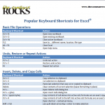
Excel Keyboard Shortcuts

Preview Excel Keyboard Shortcuts

 Hello and Welcome – to my new “Members Only” section of The Company Rocks website! 

I just published a new five-page Chart – “Popular Keyboard Shortcuts for Excel.” It is free for you to download as a PDF. 

This, along with additional content, will soon be inlcuded in my new “Exclusive Membership Content” area on my website. 

My Exclusive Membership Site is not quite ready to launch. So, I am offering this chart for you to download as a PDF from this post. 

To get this chart, click on this link –  

CR – Updated Chart of Popular Excel Keyboard Shortcuts 

New! Download My Free 50 Minute Video Recording Demonstrating Excel Keyboard Shortcuts

Click this link to learn how you can download my new “extended length” video recording. It is “free of charge!”

I am proud of the way my Excel Keyboard Shortcuts Chart turned out – and I think that you will get a lot of value out of this free resource. I organized the Keyboard Shortcuts by the following Tasks:

Excel Keyboard Shortcuts

  • Basic File Operations
  • Undo, Restore or Repeat Actions
  • Insert, Delete, and Copy Cells
  • Edit Data
  • Show / Hide Columns and Rows
  • Select Contiguous Cells
  • Navigate Within a Worksheet
  • Navigate Between Workbooks
  • Find, Replace, and Go To
  • Enter Data
  • Work with Cell Comments
  • Work with Names for Cells and Ranges
  • Work with Formulas and Functions
  • Work with Formula Precedent and Dependent Cells
  • Print Worksheet
  • Formatting Cells and Text
  • Work with Subtotals and Outlines
  • Work with Tables, Lists, and Filters
  • Work with Charts
  • Work with Excel Windows and Open Applications

So, as you can see, this is a comprehensive – but not exhaustive – list of the best Keyboard Shortcuts for Excel. I took care to ensure that these Keyboard Shortcuts will work for all versions of Excel from 2003 through version 2010. 

The 50 Best Tips

The 50 Best Tips Series

I have several video lessons that cover keyboard shortcuts on my DVD-ROM, “The 50 Best Tips for Excel 2007.” It is a best-seller and it is now on sale! Use Coupon SAVE-20-PCT at checkout and save 20% on any puchase at my online store. Click here to open a secure shopping cart

And let me know your thoughts on my Excel Keyboard Shortcut Chart. Do you have a favorite Keyboard Shortcut that you want to share with our readers? Add your comments below.

Learn how to “Master Excel in Minutes – Not Months!”

Share and Enjoy:
  • Add to favorites
  • Facebook
  • Twitter
  • Technorati
  • Print
  • email
  • Digg
  • StumbleUpon
  • del.icio.us
  • Yahoo! Buzz
  • Google Bookmarks
  • Orkut
  • SphereIt
  • Sphinn

How to Import Excel Data Into Access

This is the first in a series of lessons where I demonstrate how to integrate Excel data with an Access database. In this lesson you will learn how to:

  • Access Working with External Data

    Work with External Data

  • Import an Excel worksheet as a new Table in Access.
  • Append an Excel worksheet to the Table that we created with the Imported data.
  • Create a link between the Source Excel worksheet and an Access Table.
  • Refresh the link between Excel and Access.

First, on the Excel side of this process, make sure that you have clearly identified the Field Headers in the Top Row of your data set. If you have and cells that contain Formulas, convert the formulas to Cell Values.

Begin the Import Process

You initiate the Importing from inside Access. Go to the External Data tab on the Ribbon (in Access 2007) and choose Excel. Follow the steps in the Import Wizard. I recommend that you allow Access to create a Primary Key for the new table. This will allow you to set up “table relationships”  inside Access.

Append Excel Data to an Existing Access Table

Once you have at least one Access Table set up, you have another option when you Import Excel data – you can “Append” Excel data to the Access Table. Be sure that your “field headers” match each other. Once again, follow the steps in the Import Excel data Wizard.

Notice that with each of these Import Wizards you are given the option to save your Import definition. If you will be importing data from the same Excel source on a regular basis, this “Saved Definition” will save you a lot of time.

Link to Source Data

You can decide to establish a “link” to the source data – in this case an Excel worksheet. If you do, you will see a special “icon” next to your Access table that indicates that the table is linked to an Excel source. In this case, you can not make any changes to the tabel from inside Access. You make all changes – adding, editing and deleting records – from inside Excel.

With a link to the source data, remember to “refresh” the link to see the updated information.

Watch this Video Lesson – Embedded from YouTube

As an experiment, I am embedding this video as a YouTube Video. Click on the video and you will be watching it in High Definition, Full Screen mode on my YouTube Channel – DannyRocksExcels.

Share and Enjoy:
  • Add to favorites
  • Facebook
  • Twitter
  • Technorati
  • Print
  • email
  • Digg
  • StumbleUpon
  • del.icio.us
  • Yahoo! Buzz
  • Google Bookmarks
  • Orkut
  • SphereIt
  • Sphinn

The 10 Most Watched Videos at The Company Rocks During 2010

Reminder Note

Reminder Note

I like to look back to review the results of the past year. Which posts, which videos were the most popular, which videos were downloaded most often? As I look at this list of 10 videos, the clear winner – by category – is merging data from multiple worksheets. Three of the top 10 videos that were watch the most fall into this category!

Here is a listing of the 10 Video Lessons that were watched most frequently on my website – www.thecompanyrocks.com – during 2010:

1- Summarize Multiple Excel Worksheets – Consolidate by Position

2- Build an Accounts Receivable Aging Report

3- Use Pivot Tables to Summarize by Year, Quarter and Month

4- Simplify Data Lookups in Excel

5- Perform Break-Even Analysis with Excel’s Goal Seek Tool

6- How to Display Numbers During a PowerPoint Presentation

7- Make Excel Data Come Alive with Visualization Tools

8-  Excel 2003 Basics – Data Entry

9- How to Merge Multiple Excel Workbooks into a Master Budget

10- Consolidate Data from Multiple Excel Worksheets – Part 2 – by Category

If you enjoy these videos, you will enjoy my DVD-ROMs, “The 50 Best Tips for Excel 2007” and “The 50 Best Tips for PowerPoint 2007.” You can use my secure shopping cart to purchase them now.

I have reduced the purchase price of my Individual DVD-ROMs to $29.97 USD. You do not need a coupon to receive this special price. Simply, go to my online store – http://shop.thecompanyrocks.com

You can also watch my videos on iTunes. Click here to go to my Video Podcast, “Danny Rocks Tips and Timesavers” at the iTunes Store.

Learn how to “Master Excel in Minutes – Not Months!”

My most recent videos can be viewed in High Definition, Full Screen Mode on my YouTube Channel – DannyRocksExcels

Share and Enjoy:
  • Add to favorites
  • Facebook
  • Twitter
  • Technorati
  • Print
  • email
  • Digg
  • StumbleUpon
  • del.icio.us
  • Yahoo! Buzz
  • Google Bookmarks
  • Orkut
  • SphereIt
  • Sphinn