Excel Training | The Company Rocks

Danny June 24, 2012 Leave a Comment

How to Create Hyperlinks in Excel

One of my viewers – Ben from the UK – wrote to tell me that he needs to learn how to create Hyperlinks in Excel in preparation for a job interview this week. He asked me that, since he could not find a decent YouTube video on this topic, to create a tutorial demonstrating ow to create Hyperlinks in Excel.

Hey, in these tough economic times, I am happy to help as many people as I can. However, given my time constraints – and, my need to make a living from my video resources – I invite you to purchase one or more of my many resources on my secure online shopping website – http://shop.thecompanyrocks.com

Topics Covered in this Excel Video Tutorial

In this video tutorial, I demonstrate how to:

Create a simple Hyperlink to another worksheet in your Excel workbook
Create Hyperlinks that “Return you” to your main “Dashboard” worksheet
Hyperlink to other programs – e.g. PowerPoint
Create hyperlinks that direct a viewer to send you an E-Mail message
Hyperlinks to websites

I am the first to admit that the Insert / Edit Hyperlinks Dialog Box is confusing and “too busy” for my tastes. However, in this video tutorial, I demonstrate how to navigate through this Dialog Box and also, how to get te most out of it. For example, how to change the “text displayed” for the Hyperlink while working in the Dialog Box.

Watch this Video in High Definition

Click here – on this Hyperlink – to watch this video in High Definition on my YouTube Channel – DannyRocksExcels

View this Totorial Now!

Purchase My Resources to improve your Excel Skills

If you are in a similar situation as Ben – where you need to demonstrate specific knowledge of MS Office Programs Skills – why trust your luck? Rather, improve your skills – and your odds for securing a new job or a promotion!

I invite you to purchase one or more of my down-to-earth video tutorials. Visit my secure online shopping website – http://shop.thecompanyrocks.com

Share and Enjoy:

Filed Under: Excel Basics, Excel Training, Integrating MS Office Programs, Keyboard Shortcuts, Video Response to Viewers Tagged: Excel Dashboard with Hyperlinks, Excel Video Training, Hyperlinks, Hyperlinks to PowerPoint, Keyboard Shortcuts in Excel, Tips and Time Savers, Video lessons for Excel

Danny April 20, 2012 Leave a Comment

How to Perform Time Period Calculations in Excel

Time Calculations in Excel

Judging by the number of calls that I get from my viewers, working with Time Period Calculations is one of the most problematic challenges in Excel. My goal for this tutorial is to demonstrate how you can easily avoid the frustrations when you calculate elapsed time and total a series of time – e.g. hours worked during the week.

Apply a Custom Format to Formula Cells

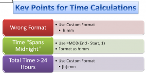
When you create an Excel Formula that subtracts a Start Time from an End Time, you are likely to get a result that looks like 2:30 AM. This is not what you want to see! The solution is to apply a Custom Time Format – e.g. h:mm – to the formula cell(s).

Time that “Spans Midnight”

Many people work the “Graveyard Shift.” The start work late in the evening and they end work early the next morning. The problem that occurs when you want to calculate the number of hours worked is that Excel believes that you are performing a “negative time” operation and the result is a cell filled with ######## (Hash Marks). This happens because Excel thinks that both the Start Time and the End Time belong in the same day. To solve this, you could use an IF() Function formula. However, there is a much easier formula to use as I demonstrate in this video. It uses the MOD() Function.

Total Hours Worked

Use the SUM() function to total 8:00 hours worked each weekday. You are expecting to see 40:00 hours worked. So why does Excel return 16:00 hours instead? By default, Excel interprets 24:00 hours as a single day. So it subtracts 24:00 from the 40:00 hours worked to return 16:00 hours. Unless you make a formatting change to the formula cell you are going to have many unhappy and under paid employees.

The solution? Apply the [h]:mm Custom Formatting to the Formula Cells. Amazingly enough, Excel does not include [h]:mm as one of the Custom Formats in the list. So, simply edit one of the other formats and you will now have the correct answer displayed for your formula!

Learn More Tips for Excel

I invite you to visit my secure online shopping website – http:shop.thecompanyrocks.com – to preview all of the resources that I offer including “The 50 Best Tips for Excel 2007” DVD-ROM.

Subscribe to the “Danny Rocks Tips and Timesavers” Video Podcast on iTunes

I offer a free video podcast for many of my video tutorials at the iTunes Store. Follow this link to see all of the Podcasts that I have posted. If you like what you see, I invite you to subscribe to this free service.

Watch Tutorial in High Definition

You can view this tutorial in High Definition on my YouTube Channel – DannyRocksExcels.

Share and Enjoy:

How to Perform Time Period Calculations in Excel [ 7:55 ] Play Now | Play in Popup | Download (1635)

Filed Under: Excel Date and Time Functions, Excel Training, Format Cells in Excel, Podcast Tips & Timesavers Tagged: Custom Formats for Time in Excel, Excel Functions, Excel Video Training, MOD() Function in Excel, time crosses midnight in Excel, Time Spans Midnight, Total Number of Hours Worked in Excel, Video lessons for Excel

Danny April 9, 2012 Leave a Comment

How to Roll Up a Summary by Month to Filter an Excel Pivot Table

Filter with a Roll Up by Month Summary

In this Excel tutorial, I respond to a viewer request. He likes the new “Roll Up Summary by Month” feature for filtering a field in an Excel 2007 – 2010 Field. What he finds frustrating – there seems to be no natural way to accomplish this with an Excel Pivot Table.

Natural Language Date Filters in Excel

Before I solve my readers dilemma, I demonstrate how to take advantage of the new “Natural Language” Date Filters that were introduced in Excel 2007. Date Filters allow you to filter records from “Today,” “Last Week,” “Next Month,” etc. They are available for Excel Tables and Excel Pivot Tables. These “Natural Language” Date Filters are a major improvement in Excel!

Group a Field for Pivot Tables

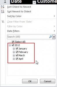
To solve my viewers question, I “Grouped” the original Date Field in his Pivot Table to produce “virtual” fields for “Month,” and “Year.” Now, it is a simple step to filter the “virtual” Month Field to obtain a “roll up” filter for individual months in the Pivot Table. Just select a single cell in the Pivot Table Date Field and choose Group Field. Make your choices in the Grouping Dialog Box and you are “good to go!”

I also show you how to take advantage of the Expand and Collapse Field Commands in a Pivot Table.

In-Depth Video Tutorial for Excel Pivot Tables

At my secure, online shopping website, you can purchase my 90-minute Video tutorial for Excel Pivot Tables. Available for immediate downloading or on a DVD-ROM. Version specific editions for Excel 2003, 2007, and 2010.

Watch Video Tutorial in High Definition

Follow this link to watch this tutorial in High Definition Mode on my YouTube Channel – DannyRocksExcels

Share and Enjoy:

How to Create a Roll Up by Month Filter for an Excel Pivot Table [ 5:42 ] Play Now | Play in Popup | Download (1696)

Filed Under: Excel Data Tables and Lists, Excel Training, Pivot Tables, Video Response to Viewers Tagged: Collapse and Expand Fields in Pivot Tables, Date Filters in Excel, Excel Pivot Tables, Excel Video Training, FIlter a List in Excel, Filter by Time Period, Group Dates in Pivot Tables, Natural Language Date Filters in Excel, Video lessons for Excel

Danny March 19, 2012 Leave a Comment

Use Conditional Formatting in Excel to Highlight Cell Values that Match Criteria

Conditional Formatting in Excel

Conditional Formatting has been available for many years in Excel. However, beginning with Excel 2007, Conditional Formatting got a major boost in its ease-of use and new visualization tools.

In this tutorial, I demonstrate how to use Conditional Formatting to highlight – via formatting – the cells in a range that anser “TRUE” to a set of criteria. For example, is the cell value “Above Average” or is it Greater than the value in a Target Cell.

How Does Conditional Formatting Work?

Conditional Formatting is “dynamic.” If you update the values – or formulas that generate cell values” the cell that receive the Conditional Formatting may change – based upon the criteria that you set as “the condition.”

Versions of Excel Covered

For this lesson, I demonstrate Conditional Formatting in BOTH Excel 2010 and Excel 2003.

Learn More About Conditional Formatting

I invite you to visit my secure online shopping website – http://shop.thecompanyrocks.com – to see all of the resources that I offer. This includes my best-selling DVD-ROM, “The 50 Best Tips for Excel 2007.”

Watch Tutorial in High Definition

Follow this link to watch this Excel Tutorial in High Definition on my YouTube Channel – DannyRocksExcels

View Tutorial Now

Share and Enjoy:

Filed Under: Conditional Formatting, Excel Training, New in Excel 2007, YouTube Videos by Danny Rocks Tagged: Conditional formatting in Excel, Excel Video Training, Video lessons for Excel

Danny March 6, 2012 1 Comment

How to Analyze Point-of-Sale Data with an Excel Pivot Table

Advantages of Pivot Tables

This is the first in a series of tutorials that I am creating in partnership with Tri-Technical Systems – a leading provider of Point-of-sale (POS) Systems. In this video lesson, I use an Excel Pivot Table to present the information that I require from a standard “Inventory by Location” report.

Point-of-Sale Reports

Most POS Systems allow you to print out standard reports – compact, professionally formatted “snapshots” of your inventory status, sales data and customer information. Likewise, most POS Systems will allow you to easily export the data behind these reports to Excel – where you can analyze or “number crunch” the data.

Advantages of Pivot Tables

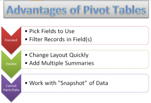
Pivot Tables combine the best elements of Subtotals, Outlines and Filtered Reports.
With a Pivot Table, you select only the Fields that you wish to focus on.
You can quickly reposition any field on your Pivot Table – e.g. change it from a Vertical to a Horizontal position.
Pivot Tables allow you to easily add multiple summaries – e.g. Sum, Average, Percentage of Total, etc. without writing a Formula!
It is impossible to harm your underlying data when you work with a Pivot Table because you are working with a “virtual snapshot” of your data. You cannot directly change any value in a Pivot Table Report!

Learn More About Pivot Tables

Pivot Tables are easy to learn. However, it does take practice if you want to really tap into the analytical power of a Pivot Table Report. Fortunately, I have a great resource for you – a 90 minute focused video tutorial on Pivot Tables. Follow this link to go to the information page for my Excel 2010 Pivot Table DVD-ROM. I have also created Pivot Table videos for Excel 2007 and Excel 2003.

Watch Tutorial in High Definition

You can watch this Excel Tutorial in High Definition on my YouTube Channel – DannyRocksExcels

View My Video Now

Share and Enjoy:

Filed Under: Excel Training, MS Excel Training, Pivot Tables Tagged: Collapse and Expand Fields in Pivot Tables, Excel Pivot Tables, Excel Video Training, Filter Fields in Pivot Tables, MS Excel Training, Using Pivot Table Report Filter

Danny March 1, 2012 Leave a Comment

How to Protect Cells that Hold Formulas in Excel

Protect Excel Formula Cells

Learning how to Protect the Excel Worksheet Cells that contain Formulas is a three-step process. This process tends to confuse and frustrate many Excel users. Some of the steps seem counter-intuitive when you first begin the process. That is why I created this video tutorial – To demonstrate each of the steps; to remove the confusion.

First, I show you how this is done in Excel 2010 / Excel 2007. Next, I show you how to protect the Formula Cells in Excel 2003.

Key Concept for Protecting Formula Cells

By default, all cells in an Excel Workbook are “Locked!”

So, if you are going to allow a user to input current values in the worksheet, you must first “select” the input cells and then, “Unlock” them.

Protecting Excel Worksheet

The final step in the process is to Protect the Worksheet. I rarely use a password for the worksheet because I tend to forget it and then I cannot even access the protected worksheet!

Take care in the Protect Sheet Dialog Box to select only the options that best suit your purpose. For example, in this video tutorial, I choose to limit users to select only the cells that I unlocked in steps 1 and 2.

Go To Special Dialog Box

The quickest way to select the cells that you wish to “unlock” is to open the Go To Special Dialog Box. There, choose “Constants.” You can limit the constants to “Numbers” as I do in this tutorial.

Danny Rocks Tips and Timesavers Podcast on iTunes

I invite you to subscribe to my “free” video podcast on iTunes. Click on this link to access all of my Podcast Videos.

Watch Tutorial in High Definition

Follow this link to view this Excel Tutorial in High Definition on my YouTube Channel – DannyRocksExcels

Share and Enjoy:

How to Protect Cells with Formulas in Excel [ 7:32 ] Play Now | Play in Popup | Download (2394)

Filed Under: Excel Formulas, Excel Training, Format Cells in Excel, Podcast Tips & Timesavers, Workbooks and Worksheets in Excel Tagged: Excel Video Training, Go To Special dialog box, MS Excel Training, Protect Excel Worksheet, Protect Formula Cells in Excel, Select Formula Cells, Tips and Time Savers, Unlock Cells in Excel Worksheet, Video lessons for Excel

Danny February 19, 2012 Leave a Comment

How to Use Named Ranges in Existing Excel Formulas

Paste Named Ranges in Formula

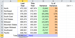
I am a strong proponent for using Named Cell Ranges when creating Excel Formulas. But what if you have already created formulas – formulas that use cell references. How do you insert or apply a newly created named range into an existing Excel Formula?

Simple answer – watch this short video to see me demonstrate how this is done.

Better answer:

Follow These Steps

Activate in-cell formula editing by either double-clicking the formula cell or using the Keyboard Shortcut F2.
Highlight the cell reference that you wish to replace with a named range.
Choose the Name from the “Use in Formulas” drop-down menu. You can also use the F3 Keyboard Shortcut to open the Paste Names Dialog Box.
Repeat these steps to complete replacing additional cell references with named cell ranges.

Learn to Get the Most from Excel

On my DVD-ROM, “The 50 Best Tips for Excel 2007,” I offer 5 1/2 hours of video instruction. You will be amazed at how much more you can get out of Excel when you invest in this valuable resource. I invite you to visit my secure, online shopping website to learn more about the resources that I offer.

Watch Video in High Definition

You can view this Excel Tutorial in High Definition on my YouTube Channel – DannyRocksExcels

Play Tutorial Now

Share and Enjoy:

Filed Under: Excel Formulas, Excel Training, Names for Cells and Ranges Tagged: Excel Keyboard Shortcuts, Excel Video Training, MS Excel Training, Named Cell in a formula, Named Cells and Ranges, Paste Names Dialog Box, Video lessons for Excel

Danny February 10, 2012 Leave a Comment

3 Reasons to Create and Use Named Ranges in Excel Formulas

Use Named Ranges in Formulas

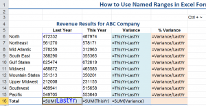
In my opinion, there are three reasons to use Named Range references in Excel Formulas:

They are easier to write. Particularly, if you are referencing cells in another worksheet.
They are easier to remember. Using =Sales – Cost of Goods Sold to determine Gross Profit vs. =A1 – B1
They are easier to explain. Especially, if you are sending an Excel Workbook to a client or a colleague.

Creating Named Ranges in Excel

In this tutorial, I demonstrate two methods for creating a named range:

Select the cells in the range and then type the name in the “Name Box” in the Upper Left Corner of the worksheet.
Select both the cell with the “Name” and the adjacent cells for the range. Then use the Keyboard Shortcut Ctrl + Shit + F3 to open the Create Names from Selection Dialog Box

Remember that all Named Ranges MUST begin with a Letter or an Underscore and they CANNOT contain any Spaces!

Paste Named Ranges into Formulas

If you are using Excel 2007 or Excel 2010, you can take advantage of Formula AutoComplete to quickly and accurately include named ranges in your formulas. In ALL versions of Excel you can use the F3 Keyboard Shortcut to open the Paste Names Dialog Box and select the named range that you wish to paste into your formula.

Additional Resources for Excel

I invite you to visit my secure online shopping website – http://shop.thecompanyrocks.com – where you can preview all of the resources that I offer you.

Watch Tutorial in High Definition

Follow this link to watch my Excel Video in High Definition. My YouTube Channel – DannyRocksExcels – has received over 1 million views!

Watch Video Now

Share and Enjoy:

Filed Under: Excel Formulas, Excel Functions, Excel Training, Names for Cells and Ranges, YouTube Videos by Danny Rocks Tagged: Excel Functions, Excel Keyboard Shortcuts, Excel Video Training, Keyboard Shortcuts in Excel, MS Excel Training, Named Cell in a formula, Named Cells and Ranges, Paste Names in Formulas, Video lessons for Excel

Danny February 7, 2012 Leave a Comment

How to Use Excel Formulas and Functions to Analyze Inventory for a Retail Store

Excel Formulas to Analyze Inventory

My friend, Alan Friedman, is a CPA and Partner in Friedman Kannenberg and Company, PC. I have been using one of the Excel Worksheets that Alan developed to teach retail store owners and managers how to analyze their inventory. In this lesson, I demonstrate how to write and copy the Excel formulas needed to perform this analysis.

Excel Formulas for Analyzing Inventory

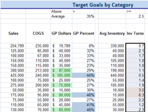
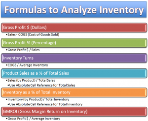
Many retailers use a Point-of-Sale (POS) System that can generate three numbers: Sales by Product Category, Cost of Goods Sold (COGS) by Product Category and Average Inventory by Product Category. Taking these three numbers – also known as “hard-coded” values – you can use Excel Formulas to give you:

Gross Profit Dollars (Sales minus COGS)
Gross Profit Percentage (Gross Profit Dollars divided by Sales)
Inventory Turns (COGS divided by Average Inventory)
Product Category Sales as a Percentage of Total Sales (Category Sales divided by Total Sales) – Use an Absolute Cell Reference
Inventory by Category as a Percentage of Total Inventory – (Inventory by Category divided by Total Inventory) – Use an Absolute Cell Reference
Gross Margin Return on Inventory (GMROI) – (Gross Profit Dollars divided by Average Inventory)

Tips for Entering and Copying Excel Formulas

As I demonstrate in this tutorial, you can write and copy an Excel Formula in one step when you first select the cells to receive the formula and use the Ctrl + Enter Keyboard Shortcut to complete the formula. Instead of clicking on the AutoSum Command or writing =SUM(), use the Alt + = (equal sign) to sum up the values in the adjacent range of cells.

Learn to Improve Your Excel Skills

If you want to learn how to create and use more Excel Formulas and Functions, I have created the Best-selling DVD-ROM, “The 50 Best Tips for Excel 2007.” You can learn more about this resource by visiting my secure online shopping website – http://shop.thecompanyrocks.com

Watch Tutorial in High Definition

I produce my Excel Tutorials in High Definition. Follow this link to view this lesson on my YouTube Channel – DannyRocksExcels

View Tutorial Now

Share and Enjoy:

Filed Under: Excel Financial Tools, Excel Formulas, Excel Functions, Excel Training, YouTube Videos by Danny Rocks Tagged: Absolute cell reference, Analyze Inventory for Retail Store, Excel Functions, Excel Video Training, Formula for GMROI, Formula for Gross Profit, Learn to use AutoFill in Excel, Video lessons for Excel

Danny February 2, 2012 Leave a Comment

The Basics for Creating and Copying Formulas and Functions in Excel

Relative and Absolute Cell References

Formulas and Functions are the “core elements” of Excel. It is vital that you have a solid grounding in understanding how formulas and functions work; especially when you need to copy and paste them into other cells.

Relative and Absolute Cell References

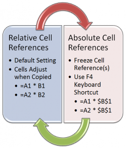
When you use Relative Cell References – the default setting in Excel – the Row numbers and Column letters adjust automatically when you copy and paste a formula.

There are, however, situations where you need to “freeze in place” part of an Excel Formula. For example, you need to “freeze” or use an Absolute Cell Reference to the cell with “Total Sales,” when creating and copying a formula to determine Product Sales as a Percentage of Total Sales.

Copying Excel Formulas

In this tutorial, I demonstrate two methods for copying and pasting formulas and functions:

Standard Practice is to select the cell with the formula and use the Ctrl + C Keyboard Shortcut to place the formula cell on the Excel clipboard. Then, after selecting the destination cell(s), use the Ctrl + V Keyboard Shortcut to paste the formula in the new location(s)
AutoFill Tool.If you are copying the formula cell into adjacent cells, use the AutoFill tool to do this quickly and accurately!

Tips that You May Not Know

In my experience, many Excel veterans are not familiar with these tips and tricks which I demonstrate in this tutorial:

The Ctrl + ~ (tilde) Keyboard Shortcut to “toggle” the Show Formulas view for the active Excel Worksheet.
The Alt + Enter Keyboard Shortcut to automatically use the =SUM() Function – for adjacent cells.
The F4 Key to automatically add Absolute Cell Reference when creating or editing a formula. For example, converts A1 to $A$1.

Learn More Excel Tips and Tricks

50 Best Tips DVD-ROM

If you enjoy the tips and techniques that I demonstrate in this lesson, then you will really benefit from purchasing my best-selling DVD-ROM, “The 50 Best Tips for Excel 2007.” You can learn more about the resources that I offer by visiting my secure online shopping website – http://shop.thecompanyrocks.com

Watch Tutorial in High Definition

Follow this link to view this Excel tutorial in High Definition on my YouTube Channel – DannyRocksExcels

Play Video Now

Share and Enjoy:

Filed Under: Excel Basics, Excel Formulas, Excel Functions, Excel Training, YouTube Videos by Danny Rocks Tagged: Absolute cell reference, AutoFill Options, AutoSum, Copy Excel Formulas, Excel Formulas, Excel Functions, Excel Keyboard Shortcuts, Excel Video Training, Keyboard Shortcuts in Excel, Learn to use AutoFill in Excel, MS Excel Training, Operators in Excel Formulas, Relative Cell Reference, Show Formulas in Excel, SUM Function in Excel, Tips and Time Savers, Video lessons for Excel

Danny Rocks “Training You to Excel”

Follow Danny on Social Media

Topics Covered in this Excel Video Tutorial

Watch this Video in High Definition

View this Totorial Now!

Purchase My Resources to improve your Excel Skills

Apply a Custom Format to Formula Cells

Time that “Spans Midnight”

Total Hours Worked

Learn More Tips for Excel

Subscribe to the “Danny Rocks Tips and Timesavers” Video Podcast on iTunes

Watch Tutorial in High Definition

Natural Language Date Filters in Excel

Group a Field for Pivot Tables

In-Depth Video Tutorial for Excel Pivot Tables

Watch Video Tutorial in High Definition

How Does Conditional Formatting Work?

Versions of Excel Covered

Learn More About Conditional Formatting

Watch Tutorial in High Definition

View Tutorial Now

Point-of-Sale Reports

Advantages of Pivot Tables

Learn More About Pivot Tables

Watch Tutorial in High Definition

View My Video Now

Key Concept for Protecting Formula Cells

Protecting Excel Worksheet

Go To Special Dialog Box

Danny Rocks Tips and Timesavers Podcast on iTunes

Watch Tutorial in High Definition

Follow These Steps

Learn to Get the Most from Excel

Watch Video in High Definition

Play Tutorial Now

Creating Named Ranges in Excel

Paste Named Ranges into Formulas

Additional Resources for Excel

Watch Tutorial in High Definition

Watch Video Now

Excel Formulas for Analyzing Inventory

Tips for Entering and Copying Excel Formulas

Learn to Improve Your Excel Skills

Watch Tutorial in High Definition

View Tutorial Now

Relative and Absolute Cell References

Copying Excel Formulas

Tips that You May Not Know

Learn More Excel Tips and Tricks

Watch Tutorial in High Definition

Play Video Now

Locate My Video Tutorials by Category

Seach My Website with Keywords

Podcast Feeds

Blogroll

Blogs for Business Writing

Blogs for Excel

Blogs for Presentations

Register or Log In

Tags