Excel Training | The Company Rocks

Danny August 24, 2011 Leave a Comment

Excel Keyboard Shortcuts to Fill a Series

Here is the latest installment in my series of video tutorials on Keyboard Shortcuts in Excel. In this lesson, I demonstrate how to Fill a Series with Values or a Formula Down or to the Right.

The more interesting Keyboard Shortcuts that I demonstrate in this lesson are:

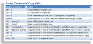
Ctrl + ‘ (apostrophe) – to copy the value from the cell directly above; to copy the formula from the cell directly above while retaining exact cell references.
Ctrl + Shift + ” (double quote) – to copy the value from the cell directly above; to copy the “result” of the formula from the cell directly above.

Download My Free “Chart of Popular Keyboard Shortcuts in Excel”

Follow this link to download all of my Popular Keyboard Shortcut Charts from my Exclusive Membership Content page.
You can also download this – for FREE – at my Online Shopping Website – here is the link: http://shop.thecompanyrocks.com/chart-of-popular-keyboard-shortcuts-for-excel/

Watch Tutorial in High Definition

Click here to go to my YouTube Channel – DannyRocksExcels – where you can watch this tutorial in High Definition mode.

Share and Enjoy:

Excel Keyboard Shortcuts to Fill a Series or Copy Values from Cell Directly Above [ 6:12 ] Play Now | Play in Popup | Download (1357)

Filed Under: Excel Training, Keyboard Shortcuts, Podcast Tips & Timesavers Tagged: Excel Keyboard Shortcuts, Excel Video Training, Fill a Series in Excel, Video lessons for Excel

Danny August 23, 2011 Leave a Comment

Excel Keyboard Shortcuts to Hide, Unhide, Insert and Delete Cells, Columns and Rows

Commands in Cells Group

Here is the latest installment in my series of video tutorials demonstrating how to use Keyboard Shortcuts in Excel. These Keyboard Shortcuts perform actions that you find in the Cells Group of commands on the Ribbon in either Excel 2007 or Excel 2010.

Topics Taught in Video Tutorial

Here are the topics that I teach in this tutorial. Using Keyboard Shortcuts to:

Select all cells in current row(s) Shift + Spacebar
Select all cells in current column(s) Ctrl + Spacebar
Open Insert Dialog Box Ctrl ++ (plus)
Open Delete Dialog Box Ctrl + – (minus)
Open short / contextual menu Shift + F10
Hide current row Ctrl + 9
Hide current column Ctrl + 0 (zero)

Download My “Chart of Popular Keyboard Shortcuts for Excel”

Click here to go to my Exclusive Membership Content page and download my charts of keyboard shortcuts. They are free to members who register.

Watch Video in High Definition

Follow this link to view this tutorial on my YouTube Channel – DannyRocksExcels

For some strange reason, I could not produce this video for my Podcast. So, the only way to view it is on YouTube.

Puchase My DVD-ROM

If you enjoy these tips. If you enjoy my style of instruction. Then, you will really benefit from purchasing and learning from my best-selling DVD-ROM, “The 50 Best Tips for Excel 2007.”

Follow this link to learn more about my DVD-ROM and to open a Secure Shopping Cart to make your purchase.

Share and Enjoy:

Filed Under: Excel Basics, Excel Training, Keyboard Shortcuts, YouTube Videos by Danny Rocks Tagged: Clear Formatting in Excel, Contextual Menu in Excel, Delete Cells in Excel, Excel Keyboard Shortcuts, Excel Short Menu, Excel Video Training, Hide Rows and Columns in Excel, Insert Cells in Excel, Insert Rows or Columns in Excel, Unhide Rows and Columns in Excel, Video lessons for Excel

Danny August 22, 2011 Leave a Comment

How to Use Excel Keyboard Shortcuts to Cut, Copy and Paste Formulas and Formatting

Keyboard Shortcuts for Cut, Copy & Paste

In addition to showing you the Keyboard Shortcuts to Cut, Copy and Paste in Excel, I demonstrate how these actions affect formulas and formatting.

Topics in this Tutorial

Here are the topics that I demonstrate in this video tutorial:

Select multiple cells using the keyboard
Use Ctrl + Enter to update all cells in the selection
Use Ctrl + ~ to “toggle” between showing and hiding formulas in all cells
Use F2 to edit in the cell – and to diagram cell references for formulas
Use Ctrl + C to copy the “relative cell references” in a formula
Use Ctrl + X to cut an Excel formula that retains the original cell references
Open and use the Office Clipboard to store up to 24 most recent copy and cut items
Use Ctrl + Z to undo multiple actions
Use Ctrl + A to select all cells in a contiguous range
Use the Delete key to delete the contents of a cell or range while retaining the formatting
Use the Clear All command to remove both formatting and contents in a range of cells

Download My Complete Charts of Popular Keyboard Shortcuts

Follow this link to my Excelusive Membership Content Page where you can download all of my charts and tables of Keyboard Shortcuts.

Watch Video in High Definition

Follow this link to view this tutorial in High Definition on my YouTube Channel – DannyRocksExcels

Share and Enjoy:

How to Use Excel Keyboard Shortcuts to Cut, Copy & Paste Formulas & Formatting [ 11:59 ] Play Now | Play in Popup | Download (1267)

Filed Under: Excel Basics, Excel Training, Format Cells in Excel, Keyboard Shortcuts, Podcast Tips & Timesavers Tagged: Clear Formatting from Cells in Excel, Copy Formulas in Excel, Excel Keyboard Shortcuts, Excel Video Training, Office Clipboard, Select Multiple Cells in Excel with Keyboard Commands, Tips and Time Savers, Video lessons for Excel

Danny August 12, 2011 3 Comments

How to Use Keyboard Shortcuts in Excel to Control Basic File Operations

Excel 2007 File Operations

If you have recently upgraded to either Excel 2007 or Excel 2010, you REALLY NEED to master the Keyboard Shortcuts that I present in this lesson!

Many Excel veterans who upgrade, tell me that they initially felt “lost” with the new user interface. Some of my clients called me in a panic because they didn’t know where to look to Print their work or to open a document. If you know how to use the Keyboard Shortcuts that I present in this lesson, you will never be at a loss. As an added bonus, these Keyboard Shortcuts work with ALL Microsoft Office programs and also for most Windows-based programs.

The “N-O-W-S” Keyboard Shortcuts

I use this acronym – NOWS – to remember the keyboard shortcuts to Open, Close and Save Documents in MS Office programs. Use Ctrl + W to Close the active worksheet.

In this video tutorial, I also show you when NOT to use Keyboard Shortcuts! There are many times when you need to access the full file menu selection.

Keyboard Shortcut for Print Preview

Use Ctrl + F2 to open up the Print Preview pane. Use the “Esc” key to Exit Print Preview.

Download My Chart of Popular Keyboard Shortcuts as a PDF

Follow this link to go to the web page where I store my Keyboard Shortcut Charts and other download-able content.

These Keyboard Shortcuts work for all versions of Excel. So far, I have found only one Keyboard Shortcut that is different when used in Excel 2007 / 2010 than in Excel 2003.

Watch Video Tutorial in High Definition Mode

Follow this link to view this video tutorial in High Definition on my YouTube Channel – DannyRocksExcels

Share and Enjoy:

Use Keyboard Shortcuts for Basic File Operations in Excel [ 10:21 ] Play Now | Play in Popup | Download (1139)

Filed Under: Excel Training, Keyboard Shortcuts, Podcast Tips & Timesavers, Workbooks and Worksheets in Excel Tagged: Excel Keyboard Shortcuts, Excel Video Training, Tips and Time Savers, Video lessons for Excel

Danny August 8, 2011 Leave a Comment

How to Customize the Quick Access Toolbar in Excel 2007

QUick Access Toolbar in Office 2007

Learning how to Customize the Quick Access Toolbar (QAT) in Excel 2007 or Excel 2010 is a great way to ease the “learning curve” when you upgrade versions.

In my experience, I have found that most people do not even realize that there is a Toolbar in Excel 2007, let alone that you can move it to a different location and to customize it!

What I Cover in this Video Tutorial

Here is what you will learn from this YouTube Video Tutorial:

To move the QAT to Show it Below the Ribbon (recommended!)
To add the most popular command buttons one at a time
To open the Customize Quick Access Toolbar Dialog Box
To find commands to add – including Command Not in the Ribbon!
To organize the commands on your QAT
To create a customized QAT for “specific workbooks” – great for special projects!
To quickly add individual command buttons with a right-click of the mours
To add entire command button groups to the QAT with a right-click of the mouse – (recommended!)

Since this video is a little longer than usual, I am making it available exclusively on my YouTube Channel.

Watch Video in High Definition Mode

Follow this Link to view this tutorial in High Definition on my YouTube Channel – DannyRocksExcels

“The 50 Best Tips for Excel 2007” DVD-ROM

Purchase my DVD-ROM, “The 50 Best Tips for Excel 2007” – on sale now at http://shop.thecompanyrocks.com for only $29.97 USD!

Share and Enjoy:

Filed Under: Excel Training, New in Excel 2007, Workbooks and Worksheets in Excel, YouTube Videos by Danny Rocks Tagged: Customize Quick Access Toolbar, Excel Video Training, Modify QAT in Excel, New in Excel 2007, Show Quick Access Toolbar below Ribbon in Excel 2007, Tips and Time Savers, Video lessons for Excel

Danny August 6, 2011 Leave a Comment

Tips to Help You Remain Productive When Upgrading to Excel 2007

Videos at the Beginning Level - 50 Best Tips for Excel

I enjoy participating in several discussion and sharing groups on LinkedIn. In one group, the question was raised, “The Ribbon – Love it or Leave it?” Many group members wrote to say that they just cannot figure out the new user interface – The Ribbon. Others expressed frustration that they were much less productive in their work as they tried to make the transition to either Excel 2007 or Excel 2010. Some said that they simply gave up and returned to using Excel 2003.

Certainly, I felt frustrated and lost when I first began to use Excel 2007. So, let me share my best tips for quickly adjusting to and mastering the commands and tools in Excel 2007 – and Excel 2010.

Topics Covered in this Video

The Office Button in Excel 2007 to open, save and print Excel workbooks and to change Excel Options
7 Standard Tabs on the Ribbon
Groups of related Command Buttons
Launchers to open up Dialog Boxes
Command Buttons with Menus
Showing the Quick Access Toolbar below the Ribbon
Customizing the Quick Access Toolbar
Working with the Mini Toolbar

Watch Video in High Definition on YouTube

Follow this link to watch this Excel Video Tutorial in High Definition on my YouTube Channel – DannyRocksExcels

Purchase My DVD-ROM, “The 50 Best Tips for Excel 2007”

Here is the link to learn more about my best-selling DVD-ROM. You can purchase this from my online store using a secure shopping cart. On sale now for only $29.97 USD.

Share and Enjoy:

Filed Under: Excel Training, MS Excel 2007 DVD, New in Excel 2007, Tips and Time Savers, YouTube Videos by Danny Rocks Tagged: Customize Quick Access Toolbar, Excel Video Training, Learning Excel 2007, MS Excel Training, New in Excel 2007, Office Button and the Ribbon in Excel 2007, Tips and Time Savers, Video lessons for Excel, Working with the Ribbon in Excel 2007

Danny July 31, 2011 Leave a Comment

Use the Show Values As Formulas in Excel Pivot Tables

Show Values As in Pivot Table

I participate in a number of Group Discussion Boards on LinkedIn. In this video tutorial, I address one question that was recently asked:

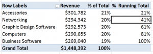
“Is it possible to show a Percentage of Running Total formula in a Pivot Table?”

The answer is, “Yes, if you are using Excel 2010. If you are using earlier versions of Excel, you can use a work-around outside the Pivot Table.”

New in Excel 2010

A great new feature introduced in Excel 2010 is the drop-down menu for the “Show Values As’ in a Pivot Table Calculation. In earlier versions of Excel, the Show Values As option was not so obvious. And, I found that many of my clients did not know how to use it – or could not locate the drop-down menu.

Work-Around for Show % of Running Total

While the “Running Total in…” calculation has been available for quite some time, the “% of Running Total in …” formula is brand new in Excel 2010. The work-around that I demonstrate is to first, create the Show As “Running Total in …” formula. Then change the Font and background of these cells to “White.” Next, write a standard formula “outside of the Pivot Table” that references these cells. Be sure to turn off the “GetPivotData” Formula when you write this formula.

Share and Enjoy:

How to Use the Show As Values Formulas in Excel Pivot Tables [ 8:13 ] Play Now | Play in Popup | Download (1325)

Filed Under: Excel Training, New in Excel 2010, Pivot Tables, Podcast Tips & Timesavers Tagged: Excel Pivot Tables, Excel Video Training, GetPivotData Function, New in Excel 2010, Pivot Table Tutorial, Show Values As in Pivot Tables, Sort Fields in Pivot Tables, Video lessons for Excel

Danny July 28, 2011 Leave a Comment

3 Work-Arounds for Shortcomings in Calculated Fields in Excel Pivot Tables

3 Work-Arounds for Calculated Fields

Don’t get me wrong. Excel Pivot Tables are a great way to summarize, analyze and present the information in your data. And, creating Calculated Fields in Pivot Tables is a terrific way to extend your analysis.

However, there are a few “quirks” that you should be aware of when using a Calculated Field”

A Calculated Field is always performed against the SUM of your data!

Well, what if you want to calculate against the MIN or the MAX of your data? Or perform some other calculation?

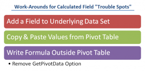
3 Work-Arounds for Calculated Field Shortcomings

I encourage you to look at a Pivot Table as “a means to an end.” Let your Pivot Table take you to the 90% completion point – and a Pivot Table does this very well! Then, use one of these 3 strategies to help you to complete your analysis.

Sometimes, you simply must return to your source data and add an additional field so that your Pivot Table has more information to work with.
You can make a copy of your Pivot Table and then Paste Special the Values to another location. From there, you can complete your analysis with more flexibility.
You can create formulas outside of the Pivot Table – as I demonstrate in this video, deselect the “pesky” GetPivotData Function first. There are some limitations here:

Remember that all cell references in your formula must appear in your Pivot Table
Your Pivot Table must essentially remain “static” – e.g. no more fields added or subtracted, etc.

Watch Video Tutorial in High Definition on YouTube

This video lesson is longer in length than normal. To watch it in High Definition, click on this link to go to my YouTube Channel – DannyRocksExcels

Download Extended Length Video Tutorials for Pivot Tables

I have created extended length video tutorial recordings for Pivot Tables in Excel 2003, Excel 2007, and Excel 2010. You can download them for only $9.95 USD.

Click on this link to get more information about my Excel Extended Length Video Recordings.

Share and Enjoy:

Filed Under: Excel Training, Pivot Tables, YouTube Videos by Danny Rocks Tagged: Calculated Fields in Pivot Tables, Excel Pivot Tables, Excel Video Training, Formulas the Reference Pivot Tables, GetPivotData Function, Paste Special, Paste Special Values, Video lessons for Excel

Danny July 25, 2011 Leave a Comment

How to Drill Down in a Pivot Table to Display the Details for a Summary Cell

Drill Down Details in Pivot Table

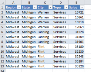
Excel Pivot Table Reports are a great way to summarize the results of multiple records in an underlying data set.

However, at some point, someone will question the accuracy of a specific calculation in your Pivot Table – this is to be expected.

When this happens. you can quickly “drill down” to display the details for any summary cell in your Pivot Table. You simply “double-click” the summary cell and you get to review the detail on a new worksheet in your Excel workbook.

Refreshing a Pivot Table

The key points to understand about Excel Pivot Tables are:

You cannot change an individual value in a Pivot Table.
You cannot update any changes from a “drill down” worksheet in a Pivot Table.
After you edit your underlying data set, you must “Refresh” your Pivot Table to get the revised calculations.

Formatting “Blank Cells” in a Pivot Table

One aspect of Pivot Tables – displaying “blank cells” – is disconcerting to many people who are using or viewing Pivot Tables for the first time. In this video tutorial, I demonstrate how to customize the display of these cells that have no underlying values to calculate.

View this Tutorial in High Definition

Follow this link to watch this video tutorial in High Defintion on my YouTube Channel – DannyRocksExcels

Master Excel Pivot Tables in 90 Minutes!

Click this link to find out how to download or purchase a DVD-ROM of my extended length video tutorials for Excel Pivot Tables.

Share and Enjoy:

Filed Under: Excel Training, Pivot Tables, YouTube Videos by Danny Rocks Tagged: Drill Dow for Details in Pivot Table, Excel Pivot Tables, Excel Video Training, Pivot Table Options, Video lessons for Excel

Danny July 20, 2011 Leave a Comment

Create a Pivot Chart to Present a Frequency Distribution Report

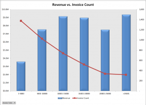
: Combination Chart for Frequency Report

Quite a few of my viewers requested that I continue my series of creating and presenting a “Frequency Distribution Report” using an Excel Pivot Table. So, here is the new Part 3 in the series!

In this Excel Video Tutorial, I demonstrate – using Excel 2010 – how to create a Pivot Chart for the Frequency Distribution Pivot Table that I created and modified in Parts 1 and 2 of this series.

Key Point: A Pivot Chart Must be based on a Pivot Table Report!

Any structural changes that you make to the Pivot Table are reflected in the Pivot Chart.
If you “filter” the Pivot Chart, those filters apply to the Pivot Table that is the basis for your Pivot Chart – and vice versa.

Focus on the Chart

As I demonstrate in this video – posted on YouTube – I prefer to focus on one task at a time. I prefer to get the formatting and structure of the Chart “right” before I think about using Filers and other “goodies to add .” This “Best Practice” helps me to get more accomplished in less time!

My bottom line is: “Focus on the task at hand. Eliminate any possible distractions from that primary task!”

A correctly designed Pivot Chart will help you to present your information accurately and interactively! For this presentation, I decided that a “Combination Chart” would be the best way to present the information that I wanted to convey. A “Combination Chart” allows you to have a Primary Axis (Revenue) that uses a Column Chart Type and a Secondary Axis (Invoice Count) that uses a Line Chart Type.

When to Use a Secondary Chart Axis

In this example, there is a wide difference between the two fields that we are charting:

Revenue for the Invoices in the “Bin Range” is in “the millions!
Count of Invoices in the “Bin Range” falls into the hundreds and low thousands.

Using a “Combination Chart” in this example – (Column Chart for Revenue in Millions) and Count of Invoices (Line Chart for Count in Hundreds) allows you to present the “relationship” between both metrics. I show you step-by-step how to create this combination chart!

Watch This Video in High Definition on YouTube

Follow this link to view this video tutorial in High Definition on my YouTube Channel – DannyRocksExcels

Click this link to view Part 1 of the 3 Part series – Creating a Frequency Distribution Report with Excel Pivot Table

Click this link to view Part 2 of the 3 Part series – Formatting a Frequency Distribution Report with Excel Pivot Table

Share and Enjoy:

Filed Under: Excel Charts, Excel Training, New in Excel 2010, Pivot Tables, YouTube Videos by Danny Rocks Tagged: Bins for Frequency Report, Combination Charts in Excel, Excel Pivot Tables, Excel Video Training, Excel Video Tutorials, Frequency Distribution Report, Group Fields in Excel Pivot Tables, Pivot Charts, video training

Danny Rocks “Training You to Excel”

Follow Danny on Social Media

Download My Free “Chart of Popular Keyboard Shortcuts in Excel”

Watch Tutorial in High Definition

Topics Taught in Video Tutorial

Download My “Chart of Popular Keyboard Shortcuts for Excel”

Watch Video in High Definition

Puchase My DVD-ROM

Topics in this Tutorial

Download My Complete Charts of Popular Keyboard Shortcuts

Watch Video in High Definition

The “N-O-W-S” Keyboard Shortcuts

Keyboard Shortcut for Print Preview

Download My Chart of Popular Keyboard Shortcuts as a PDF

More Video Tutorials for Keyboard Shortcuts

Watch Video Tutorial in High Definition Mode

What I Cover in this Video Tutorial

Watch Video in High Definition Mode

“The 50 Best Tips for Excel 2007” DVD-ROM

Topics Covered in this Video

Watch Video in High Definition on YouTube

Purchase My DVD-ROM, “The 50 Best Tips for Excel 2007”

New in Excel 2010

Work-Around for Show % of Running Total

Download Extended Length Pivot Table Video Tutorials

Watch Video in High Definition on YouTube

Master Excel Pivot Tables in 90 Minutes

3 Work-Arounds for Calculated Field Shortcomings

Watch Video Tutorial in High Definition on YouTube

Download Extended Length Video Tutorials for Pivot Tables

Refreshing a Pivot Table

Formatting “Blank Cells” in a Pivot Table

View this Tutorial in High Definition

Master Excel Pivot Tables in 90 Minutes!

Key Point: A Pivot Chart Must be based on a Pivot Table Report!

Focus on the Chart

When to Use a Secondary Chart Axis

Watch This Video in High Definition on YouTube

Locate My Video Tutorials by Category

Seach My Website with Keywords

Podcast Feeds

Blogroll

Blogs for Business Writing

Blogs for Excel

Blogs for Presentations

Register or Log In

Tags