How to Clear Cell Formatting In Excel

Numbers Stored as Text

Numbers Stored as Text

In my previous tutorial, I demonstrated how to clear all text formatting from all slides in a PowerPoint Presentation. Several viewers contacted me about publishing a tutorial that demonstrates how to clear formatting from ranges of cells in Excel.

Use the Clear Formatting Command

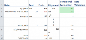
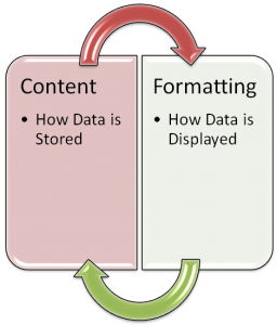
From my experience, I had found that a great many Excel users expect that formatting as well as contents are cleared when you press the Delete Key. This is not the case. The Delete Key only clears the contents of the cells in the selected range.

Use the Clear Formatting Command in the Editing Group on the Home Tab of the Ribbon. If you are using Excel 2003 or earlier, you will find this on the Edit Menu.

Numbers Stored as Text

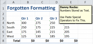
As a Best Practice, I strongly recommend that you verify that the numeric values that you will be using in formulas are truly numbers and not numbers stored as text. This, unfortunately is a common case whenever you are working with data that has been imported from a main frame computer or other external sources. In this lesson, I demonstrate how to use Paste Special Operators to quickly convert numbers stored as text to true numeric values.

9 Essential Skills for Excel 2010

9 Essential Skills for Excel 2010 Video Tutorial

Nine Essential Skills for Excel

I cover, in-depth,  Entering and formatting data as well as using Paste Special Options on my new video resource, “Nine Essential Skills for Excel.”

  • Four hours of video training
  • 25 individual video tutorials
  • Step-by-Step Instructional Guide
  • Excel Practice Files included

Download It or Order My DVD-ROM

Watch My Tutorial in High Definition

Follow this link to watch my Excel Tutorial in High Definition on my YouTube Channel – DannyRocksExcels

Share and Enjoy:
  • Add to favorites
  • Facebook
  • Twitter
  • Technorati
  • Print
  • email
  • Digg
  • StumbleUpon
  • del.icio.us
  • Yahoo! Buzz
  • Google Bookmarks
  • Orkut
  • SphereIt
  • Sphinn

Instructional Guide “9 Essential Excel 2010 Skills” – Download for Free

Instructional Guide "9 Essential Excel 2010 Skills"

Instructional Guide “9 Essential Excel 2010 Skills”

I want you to discover the scope of the Excel Training that I offer on my new video tutorial, “9 Essential Excel 2010 Skills.” So, I am offering the PDF of the Step-by-Step Instructional Guide that accompanies the video tutorial.

Link to The Company Rocks Free Resources Page

Click on this link to begin the download process for the Instructional Guide.

Instructions for Downloading the Free Instructional Guide

  1. Add this product to your secure shopping cart at my website.
  2. During Checkout, you can choose to either Register or Shop as a Guest
  3. You will need to provide a valid email address in order to receive the actual link to download my Instructional Guide.
  4. Even though you will be downloading this product, I had to set it up as a physical product with “Free Shipping.”
  5. Shortly after you complete the checkout process you will receive an email that contains a hyperlink to the file that you will download.
  6. You will be downloading a “zipped” file. So, once the download is completed, be sure to “unzip” this file!
  7. I created my Instructional Guide using the free Adobe Acrobat Reader.

Read the Instructional Guide and then Purchase my Video!

I am convinced that once you see the scope of the training in Excel 2010 that I offer, you will want to purchase the video tutorial. I offer my video in tow versions:

List of the “9 Essential Excel 2010 Skills”

9 Essential Skills for Excel 2010

9 Essential Skills for Excel 2010 Video Tutorial

These are the 9 Essential Skills that I have identified for my video tutorial:

  1. Entering Data Efficiently in Excel 2010
  2. Selecting Cell Ranges Efficiently in Excel 2010
  3. Creating and Using Named Cell Ranges in Excel 2010
  4. Applying Styles and Formatting to Excel 2010 Worksheets
  5. Working with Structured Data Sets in Excel 2010
  6. Working with Excel 2010 Formulas and Functions
  7. Using Paste Special Options in Excel 2010
  8. Using Data Validation in Excel 2010
  9. Using Excel 2010 “What-if” Analysis Tools

Excel 2010 Practice Files Included

When you purchase my video tutorial, you receive the same Excel 2010 Worksheets that I used while filming each of the 25 video tutorials. Using the same files as you view my videos, you will be able to practice your new skills. And, of course, you also receive the same Instructional Guide that I am offering for free!

I welcome your feedback! Please send me your comments via email – danny@thecompanyrocks.com – or by adding a comment below.

Thank you!


Share and Enjoy:
  • Add to favorites
  • Facebook
  • Twitter
  • Technorati
  • Print
  • email
  • Digg
  • StumbleUpon
  • del.icio.us
  • Yahoo! Buzz
  • Google Bookmarks
  • Orkut
  • SphereIt
  • Sphinn

How to Calculate the Calendar Year Quarter for a Date in Excel

Formulas to Calculate a Calendar Year Quarter

Formulas to Calculate a Calendar Year Quarter

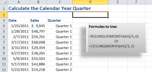
After watching my previous video tutorial, “How to Place Dates in a Fiscal Year Quarter,” several viewers requested that I demonstrate how to calculate the calendar year quarter for a date.

This requires “nesting” the MONTH() /3 Function inside either the ROUNDUP() or the CEILING() Function. I break these formulas down step-by-step in this video so that you can see how they work.

Formatting Numbers to Include Text

As a bonus, I demonstrate how to format the formula result cells to include the text “Quarter.” This is really simple to create as a custom format.

Download this Video Podcast from iTunes

You can watch and download this – and many of my – video tutorials for free at iTunes. Here is the link to my iTunes video podcast, “Danny Rocks Tips and Timesavers.”

Watch Video in High Definition

Follow this link to watch this Excel Tutorial in High Definition on my YouTube Channel – DannyRocksExcels

Visit my Secure Online Shopping Website

I invite you to visit my online shopping site – http://shop.thecompanyrocks.com – to preview and purchase my training resources. I guarantee your satisfaction 100%. I will refund your purchase if, for any reason, you are not satisfied with my products!


Share and Enjoy:
  • Add to favorites
  • Facebook
  • Twitter
  • Technorati
  • Print
  • email
  • Digg
  • StumbleUpon
  • del.icio.us
  • Yahoo! Buzz
  • Google Bookmarks
  • Orkut
  • SphereIt
  • Sphinn

How to Perform Time Period Calculations in Excel

Time Calculations in Excel

Time Calculations in Excel

Judging by the number of calls that I get from my viewers, working with Time Period Calculations is one of the most problematic challenges in Excel. My goal for this tutorial is to demonstrate how you can easily avoid the frustrations when you calculate elapsed time and total a series of time – e.g. hours worked during the week.

Apply a Custom Format to Formula Cells

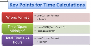
When you create an Excel Formula that subtracts a Start Time from an End Time, you are likely to get a result that looks like 2:30 AM. This is not what you want to see! The solution is to apply a Custom Time Format – e.g. h:mm – to the formula cell(s).

Time that “Spans Midnight”

Many people work the “Graveyard Shift.” The start work late in the evening and they end work early the next morning. The problem that occurs when you want to calculate the number of hours worked is that Excel believes that you are performing a “negative time” operation and the result is a cell filled with ######## (Hash Marks). This happens because Excel thinks that both the Start Time and the End Time belong in the same day. To solve this, you could use an IF() Function formula. However, there is a much easier formula to use as I demonstrate in this video. It uses the MOD() Function.

Total Hours Worked

Use the SUM() function to total 8:00 hours worked each weekday. You are expecting to see 40:00 hours worked. So why does Excel return 16:00 hours instead? By default, Excel interprets 24:00 hours as a single day. So it subtracts 24:00 from the 40:00 hours worked to return 16:00 hours. Unless you make a formatting change to the formula cell you are going to have many unhappy and under paid employees.

The solution? Apply the [h]:mm Custom Formatting to the Formula Cells. Amazingly enough, Excel does not include [h]:mm as one of the Custom Formats in the list. So, simply edit one of the other formats and you will now have the correct answer displayed for your formula!

Learn More Tips for Excel

I invite you to visit my secure online shopping website – http:shop.thecompanyrocks.com – to preview all of the resources that I offer including “The 50 Best Tips for Excel 2007” DVD-ROM.

Subscribe to the “Danny Rocks Tips and Timesavers” Video Podcast on iTunes

I offer a free video podcast for many of my video tutorials at the iTunes Store. Follow this link to see all of the Podcasts that I have posted. If you like what you see, I invite you to subscribe to this free service.

Watch Tutorial in High Definition

You can view this tutorial in High Definition on my YouTube Channel – DannyRocksExcels.


Share and Enjoy:
  • Add to favorites
  • Facebook
  • Twitter
  • Technorati
  • Print
  • email
  • Digg
  • StumbleUpon
  • del.icio.us
  • Yahoo! Buzz
  • Google Bookmarks
  • Orkut
  • SphereIt
  • Sphinn

How to Protect Cells that Hold Formulas in Excel

Protect Cells w Formulas

Protect Excel Formula Cells

Learning how to Protect the Excel Worksheet Cells that contain Formulas is a three-step process. This process tends to confuse and frustrate many Excel users. Some of the steps seem counter-intuitive when you first begin the process. That is why I created this video tutorial – To demonstrate each of the steps; to remove the confusion.

First, I show you how this is done in Excel 2010 / Excel 2007. Next, I show you how to protect the Formula Cells in Excel 2003.

Key Concept for Protecting Formula Cells

By default, all cells in an Excel Workbook are “Locked!”

So, if you are going to allow a user to input current values in the worksheet, you must first “select” the input cells and then, “Unlock” them.

Protecting Excel Worksheet

The final step in the process is to Protect the Worksheet. I rarely use a password for the worksheet because I tend to forget it and then I cannot even access the protected worksheet!

Take care in the Protect Sheet Dialog Box to select only the options that best suit your purpose. For example, in this video tutorial, I choose to limit users to select only the cells that I unlocked in steps 1 and 2.

Go To Special Dialog Box

The quickest way to select the cells that you wish to “unlock” is to open the Go To Special Dialog Box. There, choose “Constants.” You can limit the constants to “Numbers” as I do in this tutorial.

Danny Rocks Tips and Timesavers Podcast on iTunes

I invite you to subscribe to my “free” video podcast on iTunes. Click on this link to access all of my Podcast Videos.

Watch Tutorial in High Definition

Follow this link to view this Excel Tutorial in High Definition on my YouTube Channel – DannyRocksExcels


Share and Enjoy:
  • Add to favorites
  • Facebook
  • Twitter
  • Technorati
  • Print
  • email
  • Digg
  • StumbleUpon
  • del.icio.us
  • Yahoo! Buzz
  • Google Bookmarks
  • Orkut
  • SphereIt
  • Sphinn

How to use Wrap Text and Merge Cells Formatting to Improve Excel Worksheet Appearance

Wrap Text for Labels

Wrap Text for Labels

In this tutorial – the second in my series explaining how a worksheet, that my accountant friend Alan Friedman created, works – I focus on improving the formatting for the column labels and other descriptive text.

Wrap Text for Labels

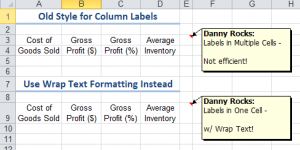
In my experience, I find that many accountants and other financial managers have not mastered the basics of formatting an Excel Worksheet. It seems that they are still using “old fashioned IBM typewriter tricks” when it comes time to create the labels for the columns of data in their spreadsheet.

Case in Point: Using two or more vertical cells to type “Cost of” (Return key on Computer) “Goods Sold.” This “old fashioned” process will lead to multiple problems. For example, improper sorting and filtering of data.

In this tutorial, I demonstrate how to use the Wrap Text command to format a single-cell text label. You will also learn how to use the Keyboard Shortcut Alt + Enter to control where your text “breaks” when wrapping text.

Merge Cells Across Columns

When you have a long, descriptive text – e.g. Your Company Name – it is best to type this into a single cell and then use the Merge Cells Command. Now, when you double-click between Column Letters to automatically expand the width of a column, only the “um-merged” labels in the column are extended in width.

Additional Resources for Tutorial

You can learn “The 50 Best Tips for Excel 2007” on my DVD-ROM. Visit – http://shop.thecompanyrocks.com/50-best-tips-for-excel-2007/ – to learn more about this.

Click on this link to download the Excel Worksheet – created by Alan Friedman – that I use in this lesson.

Watch Tutorial in High Definition

Follow this link to watch this tutorial in High Definition on my YouTube Channel – DannyRocksExcels

View Tutorial Now

Share and Enjoy:
  • Add to favorites
  • Facebook
  • Twitter
  • Technorati
  • Print
  • email
  • Digg
  • StumbleUpon
  • del.icio.us
  • Yahoo! Buzz
  • Google Bookmarks
  • Orkut
  • SphereIt
  • Sphinn

How to Apply Alternate Row Shading Using Conditional Formatting in Excel

Alternate Row Shading

Alternate Row Shading w/ Conditional Formatting

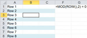
This is the first tutorial in a new series. In collaboration with my good friend, Alan Friedman – CPA and partner with the firm Friedman, Kannenberg & Co., PC – I am using Alan’s Financial worksheets to demonstrate how to get the most out of Excel. In this lesson, I show you how to apply Alternate Row Shading – aka “Green Bar Shading” – to a Year-end Inventory Analysis Excel worksheet.

Conditional Formatting in Excel

In this lesson, I create a new rule that uses a formula to determine the “condition” – or criteria – that must be met in order to apply the “formatting” to my selection of cells. The “key” to understanding this rule: The formula that you use for this “rule” must return either TRUE or FALSE. The cells – in the selection – that evaluate to TRUE will receive the special formatting – a background shading.

Extending Range of Cells to Receive Conditional Formatting

In general, you can use Excel’s AutoFill Handle to extend Conditional Formatting to adjacent cells. If, however, you want to apply the “Rule Using a Formula” to non-adjacent cells, first copy a cell that contains the Conditional Formatting. Then, use Paste Special – Formatting to apply this rule to your new selection of cells.

Resources for This Tutorial

I invite you to visit my secure online shopping website – http://shop.thecompanyrocks.com – to preview all of the resources that I offer to you.

Please visit the Friedman, Kanneberg & Co. website to download the worksheet used in this series of lessons – and other seminar handouts.


Watch Tutorial in High Definition

Follow this link to watch this Excel Tutorial in High Definition on my YouTube Channel – DannyRocksExcels

Play Video Now

Share and Enjoy:
  • Add to favorites
  • Facebook
  • Twitter
  • Technorati
  • Print
  • email
  • Digg
  • StumbleUpon
  • del.icio.us
  • Yahoo! Buzz
  • Google Bookmarks
  • Orkut
  • SphereIt
  • Sphinn

How to Clear All Underlying Cell Formatting in Excel

Clear Underlying Formatting

Clear Underlying Formatting

Have you ever typed data or a formula in a cell only to be surprised by the result? For example, you type in a number and then, unexpectedly,  Excel displays a Date or a Time in that cell. This happens frequently when you reuse an older Excel Worksheet of if you start working on a worksheet that a colleague or client has sent you.

Why does this happen?

Clear All Underlying Cell Formatting

In my experience, I have found that many Excel users mistakenly think that pressing the DELETE Key will “erase” the cells in the selection. No, No, No. The Delete key only erased the cell content – the data, text or formulas entered or pasted into the cell(s). The Delete key does NOT remove the Underlying Cell Formatting!

In this tutorial, I demonstrate how to remove the underlying cell formatting while leaving the cell Contents in place.

Topics Covered in this Tutorial

  • Using the Clear Formatting Command
  • Adding the Clear Command to your Quick Access Toolbar
  • Using Go To Special to Find and Select all cell that use either Conditional Formatting or Data Validation
  • Finding the Last Cell in your worksheet – you may be surprised to find a “remote cell” is NOT Blank!

View All the Resources that I Offer

I invite you to visit my secure online shopping website – http://shop.thecompanyrocks.com – to preview all of the resources that I offer.

Watch this Tutorial in High Definition

Follow this link to view this Excel Tutorial in High Definition on my YouTube Channel – DannyRocksExcels


Share and Enjoy:
  • Add to favorites
  • Facebook
  • Twitter
  • Technorati
  • Print
  • email
  • Digg
  • StumbleUpon
  • del.icio.us
  • Yahoo! Buzz
  • Google Bookmarks
  • Orkut
  • SphereIt
  • Sphinn

Tips for Creating 52 Weeks of Employee Time Cards in Excel

Insert & Copy Worksheets

Insert & Copy Worksheets

We are now winding down the end of the year 2011. Several of my viewers and clients have asked my for help in creating one Excel Workbook that will contain 52 weeks of employee time card information:

  • Name and Department of Employee
  • Hours Worked each day of the week – Regular and Overtime
  • Number of Holiday / Sick Days that were used / that remain, etc.

First Tutorial in this Series

Rather than trying to create each individual – and some are very specific – request, I have decided to combine multiple requests into a series of Best Practice Tips for my general audience to consider.

In this lesson, I demonstrate:

  • Two methods for adding new blank worksheets to the Excel workbook
  • Two Methods for inserting an exact copy of an existing – and formatted – worksheet
  • My favorite tip – Fill Across Worksheets – either the formatting only, the contents only or the default setting – both formatting and contents.

Links to Additional Tutorials in this Series

Watch Tutorial In High Definition

Follow this link to watch this tutorial in High Definition on my YouTube Channel – DannyRocksExcels

Additional Resources at My Online Shopping Website

I invite you to visit my new – secure – online shopping website – http://shop.thecompanyrocks.com – and preview the many tutorials and resources that I offer you.

Watch Tutorial Now

Share and Enjoy:
  • Add to favorites
  • Facebook
  • Twitter
  • Technorati
  • Print
  • email
  • Digg
  • StumbleUpon
  • del.icio.us
  • Yahoo! Buzz
  • Google Bookmarks
  • Orkut
  • SphereIt
  • Sphinn

How to Distinguish Cell Content from Cell Formatting in Excel

Cell Content vs Cell Formatting

Cell Content vs. Cell Formatting

Many Excel Users are surprised to discover that the Delete Key does not clear the formatting for the selected cell or range of cells. This can cause some unusual “surprises” you you or one of your colleagues later uses this “Deleted” Cell Range!

On the other hand, some cells must be formatted properly in order to return the correct result. This is especially true for cells that contain Time and Date Calculations. For example, in order to properly calculate a Sum of Hours that exceeds 24 hours, you need to apply the Custom Format [h]:mm to the formula cell.

Topics Taught in this Tutorial

  • Adding the Clear Command to the Quick Access Toolbar (QAT).
  • Using Go To Special – Last Cell, to find the last cell in the worksheet that contains either content or formatting – or both!
  • Understanding how Excel Stores Dates (as a Serial Number) and Times (as a Decimal Number) vs. How you use Cell Formatting to make Dates & Times easier to understand.
  • Using Keyboard Shortcuts to add the Current Date – Ctrl + ; (semi-colon) or Current Time -Ctrl + Shift + : (colon), or to “Toggle” between Formulas and Displayed Results  -Ctrl + ~ tilde).

Visit My New, Secure Online Shopping Website

Stop by http://shop.thecompanyrocks.com to see the new products that I have created. You can also download – for FREE – my Chart of Popular Excel Keyboard Shortcuts when you visit.

Watch Tutorial in High Definition

Follow this link to view this Excel Tutorial in High Definition on my YouTube Channel – DannyRocksExcels

YouTube Tutorial for this Post

Share and Enjoy:
  • Add to favorites
  • Facebook
  • Twitter
  • Technorati
  • Print
  • email
  • Digg
  • StumbleUpon
  • del.icio.us
  • Yahoo! Buzz
  • Google Bookmarks
  • Orkut
  • SphereIt
  • Sphinn