How to Use Excel Formulas and Functions to Analyze Inventory for a Retail Store

Excel Formulas to Analyze Inventory

Excel Formulas to Analyze Inventory

My friend, Alan Friedman, is a CPA and Partner in Friedman Kannenberg and Company, PC. I have been using one of the Excel Worksheets that Alan developed to teach retail store owners and managers how to analyze their inventory. In this lesson, I demonstrate how to write and copy the Excel formulas needed to perform this analysis.

Excel Formulas for Analyzing Inventory

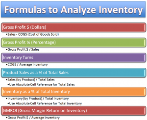
Many retailers use a Point-of-Sale (POS) System that can generate three numbers: Sales by Product Category, Cost of Goods Sold (COGS) by Product Category and Average Inventory by Product Category. Taking these three numbers – also known as “hard-coded” values – you can use Excel Formulas to give you:

  • Gross Profit Dollars (Sales minus COGS)
  • Gross Profit Percentage (Gross Profit Dollars divided by Sales)
  • Inventory Turns (COGS divided by Average Inventory)
  • Product Category Sales as a Percentage of Total Sales (Category Sales divided by Total Sales) – Use an Absolute Cell Reference
  • Inventory by Category as a Percentage of Total Inventory – (Inventory by Category divided by Total Inventory) – Use an Absolute Cell Reference
  • Gross Margin Return on Inventory (GMROI) – (Gross Profit Dollars divided by Average Inventory)

Tips for Entering and Copying Excel Formulas

As I demonstrate in this tutorial, you can write and copy an Excel Formula in one step when you first select the cells to receive the formula and use the Ctrl + Enter Keyboard Shortcut to complete the formula. Instead of clicking on the AutoSum Command or writing =SUM(), use the Alt + = (equal sign) to sum up the values in the adjacent range of cells.

Learn to Improve Your Excel Skills

If you want to learn how to create and use more Excel Formulas and Functions, I have created the Best-selling DVD-ROM, “The 50 Best Tips for Excel 2007.” You can learn more about this resource by visiting my secure online shopping website – http://shop.thecompanyrocks.com

Watch Tutorial in High Definition

I produce my Excel Tutorials in High Definition. Follow this link to view this lesson on my YouTube Channel – DannyRocksExcels
View Tutorial Now

Share and Enjoy:
  • Add to favorites
  • Facebook
  • Twitter
  • Technorati
  • Print
  • email
  • Digg
  • StumbleUpon
  • del.icio.us
  • Yahoo! Buzz
  • Google Bookmarks
  • Orkut
  • SphereIt
  • Sphinn

The Basics for Creating and Copying Formulas and Functions in Excel

Relative and Absolute Cell References

Relative and Absolute Cell References

Formulas and Functions are the “core elements” of Excel. It is vital that you have a solid grounding in understanding how formulas and functions work; especially when you need to copy and paste them into other cells.

Relative and Absolute Cell References

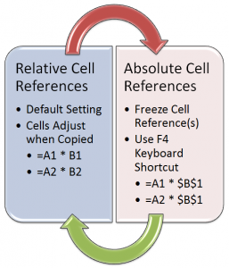
When you use Relative Cell References – the default setting in Excel – the Row numbers and Column letters adjust automatically when you copy and paste a formula.

There are, however, situations where you need to “freeze in place” part of an Excel Formula. For example, you need to “freeze” or use an Absolute Cell Reference to the cell with “Total Sales,” when creating and copying a formula to determine Product Sales as a Percentage of Total Sales.

Copying Excel Formulas

In this tutorial, I demonstrate two methods for copying and pasting formulas and functions:

  • Standard Practice is to select the cell with the formula and use the Ctrl + C Keyboard Shortcut to place the formula cell on the Excel clipboard. Then, after selecting the destination cell(s), use the Ctrl + V Keyboard Shortcut to paste the formula in the new location(s)
  • AutoFill Tool.If you are copying the formula cell into adjacent cells, use the AutoFill tool to do this quickly and accurately!

Tips that You May Not Know

In my experience, many Excel veterans are not familiar with these tips and tricks which I demonstrate in this tutorial:

  • The Ctrl + ~ (tilde) Keyboard Shortcut to “toggle” the Show Formulas view for the active Excel Worksheet.
  • The Alt + Enter Keyboard Shortcut to automatically use the =SUM() Function – for adjacent cells.
  • The F4 Key to automatically add Absolute Cell Reference when creating or editing a formula. For example, converts A1 to $A$1.

Learn More Excel Tips and Tricks

50 Best Tips for Excel 2007

50 Best Tips DVD-ROM

If you enjoy the tips and techniques that I demonstrate in this lesson, then you will really benefit from purchasing my best-selling DVD-ROM, “The 50 Best Tips for Excel 2007.” You can learn more about the resources that I offer by visiting my secure online shopping website – http://shop.thecompanyrocks.com

Watch Tutorial in High Definition

Follow this link to view this Excel tutorial in High Definition on my YouTube Channel – DannyRocksExcels

Play Video Now

Share and Enjoy:
  • Add to favorites
  • Facebook
  • Twitter
  • Technorati
  • Print
  • email
  • Digg
  • StumbleUpon
  • del.icio.us
  • Yahoo! Buzz
  • Google Bookmarks
  • Orkut
  • SphereIt
  • Sphinn

Tips for Working with Array Formulas and Functions in Excel

Using ARRAY Functions in Excel

ARRAY Formulas in Excel

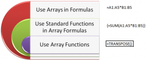
Array Formulas and Functions are very powerful tools to use in Excel. However, the concept of working with ARRAYs take a little bit of time and practice. In this video tutorial, I demonstrate how to:

  1. Create formulas that use ARRAYS as arguments
  2. Work with ARRAY FUNCTIONS – for example, the TRANSPOSE Function
  3. Key “Got’cha” steps to master – for example, selecting all cells to receive formula results before creating the ARRAY Formula.
  4. The importance of using Ctrl+Shift+Enter to complete the Array formula.

What is an ARRAY?

“An Array is a collection of Cells or Values that Excel treats as a single unit.”

Why Use an ARRAY Formula?

  1. Automatic Level of Protection for Formula Cells – You cannot delete nor edit a single cell in an Array Formula
  2. Eliminate Intermediary Calculations – For example, you can find the Grand Total without having to create a field to calculate “Extended Price.”
  3. Worksheet, usually, calculates faster because you are using fewer formulas.

Visit My NEW Online Shopping Website

http://shop.thecompanyrocks.com is my new, secure online shopping website. I invite you to visit and preview my new products.

Watch Tutorial in High Definition

Follow this link to view this tutorial in High Definition on my YouTube Channel – DannyRocksExcels

Share and Enjoy:
  • Add to favorites
  • Facebook
  • Twitter
  • Technorati
  • Print
  • email
  • Digg
  • StumbleUpon
  • del.icio.us
  • Yahoo! Buzz
  • Google Bookmarks
  • Orkut
  • SphereIt
  • Sphinn

Structured Formula References in Excel 2007 and Excel 2010 – Part 2

Compare Structered References Excel 2007 v 2010

Compare Structured References 2007 v 2010

This is the second and concluding part of this series where I demonstrate how to use Structured Formula References when referring to Excel Tables.

Key Points Covered

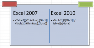
  • The difference between Structured Formula References in Excel 2007 and Excel 2010
  • How to Edit Structured Formula References
  • How to Write Structured Formulas using the new Formula AutoComplete drop-down menu


Watch My Video Tutorial Now


Watch Video in High Definition on YouTube

Click on this link to watch this Video in High Definition on my YouTube Channel – DannyRocksExcels

Go to Part 1 in this Series of Video Tutorials

Follow this link to go to Part 1 in this Series of Tutorials about using Structured Formula References in Excel Tables.

Visit My New Secure Online Store

I have just published 6 New Products and opened a new, revised, secure online shopping website. Take a look at: http://shop.thecompanyrocks.com


Share and Enjoy:
  • Add to favorites
  • Facebook
  • Twitter
  • Technorati
  • Print
  • email
  • Digg
  • StumbleUpon
  • del.icio.us
  • Yahoo! Buzz
  • Google Bookmarks
  • Orkut
  • SphereIt
  • Sphinn

How to Take Advantage of the Go To Special Dialog Box Options in Excel

Go To Special Options

Go To Special Options

In my opinion, the Go To Special Options Dialog Box offers some of the most useful tools in Excel!

Why?

Because,  you must…

Select Cells Before Performing an Action on these Cells

The “key” to understanding ANY MS Office or Windows Program is… You MUST select a single cell or a range of cells BEFORE you can perform an action on them – e.g. Formatting you selection, deleting your selection, editing your selection or auditing your selection.

Tips Presented in this Video Tutorial

  • Select cells with Comments – so that you can “format” these cells to make them easier to identify.
  • Select cells that contain Constant Numeric Values – so that you can easily “spot” cells that should – bu do not – contain formulas.
  • Select cells that contain Specific Types of Formulas – e.g. Text Formulas – to “audit” your formulas.
  • Find the “Last Cell” in your worksheet – the last cell that contains EITHER content OR FORMATTING – This can be an “eye-opener!” for you.
  • Select the cells that contain Data Validation – perhaps you failed to “validate” all of the cells in a range.
  • Select the cells that contain Conditional Formatting – perhaps your did not select ALL of the cells in a Range BEFORE you applied a Conditional Formatting RULE!
  • Learn how to select the “Visible Cells Only” before performing a copy and paste operation – especially helpful when copying the “collapsed cells” for an Excel Outline.

I am positive that Excel users at ANY LEVEL will be able to pick up at least one solid tip from this Video Tutorial. Please send me your comments to let me know what you learned – or what you need clarification on.

Watch Tutorial in High Definition Mode

Follow this link to view this Excel Tutorial in High Definition / Full Screen Mode on my YouTube Channel – DannyRocksExcels

Learn About My New Extended Length Excel Video Tutorials

I have just published the first in a series of “Extended Length” – 90 Minutes – Video Tutorials, “Excel Pivot Tables to Summarize, Analyze and Present Your Data.” Follow this link to learn more about this tutorial. I have created separate versions of the tutorial for Excel 2010, 2007 and 2003.

Share and Enjoy:
  • Add to favorites
  • Facebook
  • Twitter
  • Technorati
  • Print
  • email
  • Digg
  • StumbleUpon
  • del.icio.us
  • Yahoo! Buzz
  • Google Bookmarks
  • Orkut
  • SphereIt
  • Sphinn

How to Use an Excel Macro to Quickly Fill in Blank Cell Labels

Options for Filling in Blank Cell Labels

Options for Filling in Blank Cell Labels

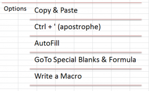
In this Excel video tutorial, I demonstrate how to write, proofreed and run a Macro that will quickly fill in values for blank cell lables in a report that you may have received from a colleague or a client.

Reports With “Holes in the Data”

Frequently, when you receive a report that was created in an Excel Pivot Table or from a relational database – e.g. MS Access – the report looks great! However, if you wish to apply filters or other analysis to this report, you will need to fill in the “missing” or blank cell labels.  

Watch This Excel Video Tutorial in High Definition

Follow this link to view this lesson in High Definition, Full Screen Mode on my YouTube Channel – DannyRocksExcels

Related Excel Video Tutorials

If you would like to learn how to convert an Excel Pivot Table to a Standard List – and to Fill in the Blank Cell Labels – click on this link to see my video tutorial on this topic.

And, here is a link to another related Excel Video Tutorial – Quickly Fill in Blank Cell Labels

Share and Enjoy:
  • Add to favorites
  • Facebook
  • Twitter
  • Technorati
  • Print
  • email
  • Digg
  • StumbleUpon
  • del.icio.us
  • Yahoo! Buzz
  • Google Bookmarks
  • Orkut
  • SphereIt
  • Sphinn

How to Convert a Pivot Table to a Standard List

Watch this video tutorial in High Definition on YouTube

A viewer aksed for my help. She has a boss and a few customers who:

  1. Do not know how to create or use Pivot Tables
  2. Have no desire to learn how to create and use Pivot Tables
Convert Pivot Table to Standard List

Convert Pivot Table to List

Nevertheless, in this example, she is being asked to create a summary report – by Year and by Quarter – from @ 5,000 daily transaction records. The fastest way to create this report is with a Pivot Table. Now, to meet the demands of her boss and clients, she needs to convert this Pivot Table into a standard list that can be Filtered and Subtotaled.

Summarize by Year and Quarter

To create this Pivot Table report:

  • Add the “Date” field to the grid and then select a single date.
  • Group the Date field by Month, Quarter and Year.
  • Add and arrange the Customer and Invoice fields to the Pivot Table Grid.

Convert Pivot Table to Standard List

  1. Remove both the Subtotals and Grand Totals from the Pivot Table Report.
  2. In Excel 2007 & 2010, ensure that you are using either the Outline or Tabular report layouts – NOT the new “default” Compact layout.
  3. Also in Excel 2007 & 2010, remove the Field Headers and the + / – Symbols.
  4. Now, select the entire Pivot talbe (use Ctrl + A) and copy it to the clipboard.
  5. Use Paste Special Values to paste the Pivot Table Results.

Filling the Blank Cells in the List

As you can see, whenever you have “nested rows” in a Pivot Table you get a nice, clean report. However, in order to Filter and Subtotal this new list, you will need to “fill in the blank cells.”

  1. Select all of the values and all of the blanks in Column A.
  2. Use Ctrl + G (or F5) to open the Go To Dialog Box and choose Special.
  3. From the Go To Special choices choose “Blanks.”
  4. With all of the Blank Cells selected use this formula: = ↑
  5. Do NOT press Enter. Rather, press Ctrl + Enter and all of the Blank Cells are now filled in with the Customer Names!
  6. Finally use Copy, Paste Special, Values to complete this process.

Watch This Video on My YouTube Channel – DannyRocksExcels

Since this video tutorial is a little longer than usual, I have decided to post it as a video – in High Definition – on my YouTube Channel. Click here to view it or copy and paste this link into your browser:

Link to YouTube Video:   http://youtu.be/IwReVDJ7BAI?hd=1

Download This Excel Workbook

Share and Enjoy:
  • Add to favorites
  • Facebook
  • Twitter
  • Technorati
  • Print
  • email
  • Digg
  • StumbleUpon
  • del.icio.us
  • Yahoo! Buzz
  • Google Bookmarks
  • Orkut
  • SphereIt
  • Sphinn

Dynamically Update a Cell with an Excel Worksheet Name

Formula to Capture Worksheet Name

Capture Tab Name in Cell

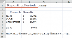
I am excited to share this Excel Tip with you! Several viewers have recently asked if there was a way to create a link in a cell to the name of a worksheet tab. Yes there is! And, in this lesson, I demonstrate how to do this.

Say, for example, that you want Cell C1 to contain the name of the current worksheet (Sheet1). With this formula, when you change the name of the worksheet to “January,” cell C1 is dynamically updated to show “January.”

Perfect for Excel Templates

If you use a template for your monthly, regional sales or financial reports, then this Excel formula is essential. You write the formula once – using Group edit – and each worksheet in your Excel workbook will be linked to a cell in your report. Change the name of the worksheet and your report name is automatically updated.

Functions Used in this Formula

  • CELL() – to gather information about the worksheet – in this case, the “Filename.”
  • MID() – to extract the characters in a text string – e,g, the “worksheet name.”
  • FIND() – to locate the starting point for the MID() function to extract the characters in the text.

As the final argument for the MID() Function, I use 31 characters because that is the maximum number of characters that you can use when naming an Excel worksheet.

Try this for yourself. Let me know how it works for you. Add your comments below.

Download Excel Workbook for this Lesson

Watch Video in High Definition

Follow this link to view this video tutorial on my YouTube Channel – DannyRocksExcels

I invite you to watch or to subscribe to my video podcast on iTunes. Follow this link to learn more about my RSS Feed.

Share and Enjoy:
  • Add to favorites
  • Facebook
  • Twitter
  • Technorati
  • Print
  • email
  • Digg
  • StumbleUpon
  • del.icio.us
  • Yahoo! Buzz
  • Google Bookmarks
  • Orkut
  • SphereIt
  • Sphinn

Learn How Excel Calculates Formulas

Order of Calculations in Excel

Excel Calculation Order

Have you ever written a Formula in Excel only to receive a result that was different from the one you expected? Most Excel users have shared that experience from time to time! Excel is smart and fast. However, it can not read your mind.

In this lesson, I show you how Excel evaluates and calculates a formula. Once you understand “Excel’s perspective” of the formula, you will know how to correctly write the formula so that Excel will produce the result that you intended. In other words, to see the formula from “your perspective!

Order of Precedence

Excel performs calculations in formulas moving from left to right in this order:

  1. Performs Multiplication (*) and Division (/)
  2. Goes back and performs Addition (+) and Subtraction (-)

This is the “key” to consistently getting Excel to produce the results that you intended. No, you can’t get Excel to make you an “instant millionaire” or do anything illegal. However, understanding how to write formulas correctly – so that you control the order of calculation in Excel – is the “secret sauce!”

Control the Order of Calculation in Excel This formula: =5+15*2 results in 35. If you were expecting the result to be 40, then write the formula as (5+15)*2. In other words, take the “result” of 5+15 or 20 and multiply this by 2 to give me 40.By using parentheses (5+15) you take control over the order of precedence that Excel uses. Help Excel to see the formula from your perspective!

Free Chart of Excel Formula Operators

I have published  a chart – “Using Operators in Excel Formulas” – To get your free copy as a PDF, click on the link below:

CR – Using Operators in Excel Formulas

Explore My Free Excel Video Lessons

Follow this link to my Index of Free Excel Video Tutorials

Watch This Video Tutorial In High Definition

This link will take you to the DannyRocksExcels video on YouTube

Share and Enjoy:
  • Add to favorites
  • Facebook
  • Twitter
  • Technorati
  • Print
  • email
  • Digg
  • StumbleUpon
  • del.icio.us
  • Yahoo! Buzz
  • Google Bookmarks
  • Orkut
  • SphereIt
  • Sphinn

Create Dynamic Chart Titles in Excel

A viewer wrote to ask for my help in creating dynamic chart titles in Excel. He has created a series of pivot table reports and pivot charts. He wants the titles for his charts to update dynamically. That is, as he selects a new filter for his pivot table, he wants the title in his pivot chart to match the value label in his filter.

Dynamic Chart Titles


Note: 

This technique will work for all Excel Charts and Chart Types. It is not restricted to Pivot Tables.

The solution is rather simple: You link the Chart Title to a formula.

Link Chart Title to Formula

Select a cell that is outside the range of your Pivot Table – let’s say cell H1. An example formula is:

=”Sales for Fiscal Year “&D1

In this case, cell D1 contains the label for the value that you are selecting to filter your Pivot Table Report and Chart – e.g. 2008 as your Fiscal Year.

Notice that in the formula, I include the “TEXT” inside ” ” (double quotation marks. I also use the & (ampersand) to join the text to the cell reference (D1).

Finally, select the Chart Title and then, in the formula bar type =H1 (where H1 is the cell that contains the formula that we just wrote).

As a finishing touch, you can “hide” the formula in cell H1 by changing the FONT COLOR to match the background color for that cell.

It is that easy! Try it yourself after you watch this short (6 minutes) video lesson.

Invitation to Visit My New Online Shopping Site

Shop for The 50 Best Tips for Excel 2007

Shop for The 50 Best Tips for Excel 2007

My new, secure, online shopping website – http://shop.thecompanyrocks.com – is now open. I invite you to stop by for a visit and get more information about the many resources  that I offer for sale including, “Learn how to “Master Excel in Minutes – Not Months!”

Watch Tutorial in High Definition

Follow this link to my YouTube Channel – DannyRocksExcels – where you can watch this video lesson in High Definition, Full-screen mode.

Share and Enjoy:
  • Add to favorites
  • Facebook
  • Twitter
  • Technorati
  • Print
  • email
  • Digg
  • StumbleUpon
  • del.icio.us
  • Yahoo! Buzz
  • Google Bookmarks
  • Orkut
  • SphereIt
  • Sphinn