Use SumIf and SumIfs Function in Accounts Receivable Status Report

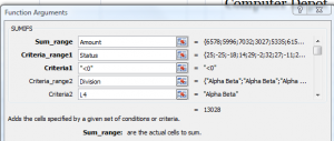
I receive many requests from viewers to help them to create and to analyze “Accounts Receivable Reports.” So, I created this Excel Video tutorial to demonstrate how both the SUMIF and the SUMIFS Functions can help you to analyze the data in an AR Status Report.

The SUMIF() Function has been available for many years in Excel – and it is a great function to use. However, starting in Excel 2007, we now have the expanded SUMIFS Function which allows us to evaluate multiple ranges using multiple criteria to return the sum of our results. This is a terrific improvement!

SUMIFS Function

SUMIFS in Excel 2007

Use SUMIFS() Function

With the SUMIFS Function, you no longer have to create multiple, complicated “nested IF Functions. Rather. you use a series of “paired arguments” – Criteria Range1, Criteria1″ etc. to define the result that you want to return.

So, with the SUMIFS() Function, you can use “paired” Criteria Ranges and Criteria to produce the exact results that you are seeking!

This, alone, may be one of the reasons to upgrade to either Excel 2007 or to Excel 2010!

Watch this Video in High Definition mode on YouTube

Here is the link to view this Excel lesson in High Definition on my YouTube Channel

You can learn how to “Master Excel in Minutes – Not Months!”

Share and Enjoy:
  • Add to favorites
  • Facebook
  • Twitter
  • Technorati
  • Print
  • email
  • Digg
  • StumbleUpon
  • del.icio.us
  • Yahoo! Buzz
  • Google Bookmarks
  • Orkut
  • SphereIt
  • Sphinn

How to Use the Average Functions in Excel 2007 and 2010

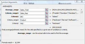
The new AVERAGEIF and AVERAGIFS Functions were introduced in Excel 2007. In this lesson, I demonstrate how and when to use both functions. If you are using an earlier version of Excel – e.g. Excel 2003, I show you how to use a Pivot Table to produce the same results.

Average is not the Median

The Average Function is the “Arithmetic Mean” of the range of cell values. This means the Sum of the values in the range divided by the Count of the cells with numeric values in the range. Many people confuse this with the MEDIAN sale which is the “middle value” in the range. Half of the cell values are above and half of the cell values are below the result of the MEDIAN() Function.

New AverageIfs Function in Excel

AverageIfs Function

New Functions in Excel 2007

Watch the video to see how to use both the AverageIf and AverageIfs Functions. I recommend using the Function Arguments Dialog Box and Named Cell References with these functions. Pay attention to my use of “Mixed Cell References” in the AverageIfs formula. Doing so makes it easy to write the formula in one cell and then copy it across the range of cells.

Here is the link to watch this video tutorial in High Definition on my YouTube Channel.

Learn how you can “Master Excel in Minutes – Not Months!”

Share and Enjoy:
  • Add to favorites
  • Facebook
  • Twitter
  • Technorati
  • Print
  • email
  • Digg
  • StumbleUpon
  • del.icio.us
  • Yahoo! Buzz
  • Google Bookmarks
  • Orkut
  • SphereIt
  • Sphinn

Create a Pivot Table for a Water or Hydrological Year

A viewer asked for my help in creating a Pivot Table Report that is based on a Water Year – also known as a Hydrological Year. In North America, a Water Year begins on October 1 and ends on September 30. If you use a Fiscal Year in your reporting, you will want to watch this Excel Training Video Lesson.

Pivot Table for Water Year

Pivot Table for Water Year

Add Two Fields to Source Data

In order for a Pivot Table to summarize non-calendar years and quarters you will need to have two additional fields in your source data:

  1. A Fiscal Year (Water Year) Field – Use the IF(), MONTH() and YEAR() Functions to produce this.
  2. A Fiscal Quarter (Hydrological) Quarter Field – Use the CHOOSE() Function to produce this.

Now you are ready to create your Pivot Table Report.

Group Dates by Month and Year

Begin by grouping the Date Field by Month and Year – not, in this case, by Quarter. Now, remove the new Year field that you just created and add in the Water Year Field and the Hydrological Quarter to the Pivot Table. Continue to arrange the Pivot Table to suit your needs.

Since there is no direct way to change a Calender Year into a Fiscal Year or Water Year, you must prepare your data prior to beginning to create your Pivot Table. Now that you have watched this video lesson, you know how to do this!

Learn how to “Quickly Create Excel Pivot Tables and Charts”

Related Excel Video Lessons

Follow this link to watch this video in High Definition mode on my YouTube Channel – DannyRocksExcels

Share and Enjoy:
  • Add to favorites
  • Facebook
  • Twitter
  • Technorati
  • Print
  • email
  • Digg
  • StumbleUpon
  • del.icio.us
  • Yahoo! Buzz
  • Google Bookmarks
  • Orkut
  • SphereIt
  • Sphinn

How to Find and Change Numbers Stored as Text in Excel

Whenever a client or a colleague sends me an Excel workbook I like to inspect it, to be sure that the “numbers are really numbers.” I will not get accurate results when I SUM them if there are some cells that appear to contain numbers, but really display a “number stored as text.”

Prevent GIGO

Prevent GIGO

This is an example of GIGO – “Garbage in delivers Garbage Out!” I take steps to prevent an outbreak of GIGO in my Excel worksheets.

Looking for Numbers Stored as Text

As a best practice, I use both the COUNT() Function and the COUNTA() function to see if there is a difference between the number of cells with numbers (the COUNT Function) and the number of non-blank cells (the COUNTA Function). In this example, I was expecting to see 31 cells with numbers in the range of sales. There were on 27. So, I need to find those 4 cells that contain “numbers stored as text.” 

If you have a keen eye – and some time to spare – you can look for cells with a little Green triangle in the upper left corner. Click on the message next to these “marked” cells and read the error message. Excel will offer to correct the error – one cell at a time. That is not an efficient way to proceed!

Use the ISTEXT() or ISNUMBER() Functions

An alternative way to find the cells that contain text stored as numbers is to use one of the “logical functions” ISTEXT or ISNUMBER. Each returns either TRUE or FALSE when evaluating a cell. You can then sort the data to group the TRUE results together and then change them – again, one at a time. This is also not the best way to make the changes.

Use Conditional Formatting to Highlight Cells with Number Stored as Text

I like to use the ISTEXT() Function as a “Rule” to apply special formatting to the cells that evaluate as TRUE with Conditional Formatting. Be sure that you select the cells that you want to evaluate before applying the Conditional Formatting.

Use Paste Special – Add

The quickest way to change numbers stored as text into real numbers is to use Paste Special – Add. First, select and copy a blank cell. Next, select your data range – in this case the cells with “Sales.” Then, right click the selection and choose Paste Special. In the dialog box select “Add.” Now – instantly – all of the cells with numbers stored as text have been changed into real numbers. You have stamped out GIGO!

Learn how to “Master Excel in Minutes – Not Months!”

Follow this link to watch this video in High Definition, Full-screen mode on my YouTube Channel – DannyRocksExcels

Share and Enjoy:
  • Add to favorites
  • Facebook
  • Twitter
  • Technorati
  • Print
  • email
  • Digg
  • StumbleUpon
  • del.icio.us
  • Yahoo! Buzz
  • Google Bookmarks
  • Orkut
  • SphereIt
  • Sphinn

Working With Array Formulas in Excel

There are at least two benefits to using an Array Formula in Excel:

  1. They will speed up creating your formulas by, in many cases, eliminating intermediate formulas.
  2. They will add a level of protection to your formulas because you cannot edit the individual cells in an Array Formula. You must edit “all” of the cells.
Array Formulas
Array Formulas

In this lesson, I first demonstrate how to select and use arrays with the SUMPRODUCT() Function in Excel. SUMPRODUCT is a very handy function to use when you want to first multiply (PRODUCT) the cells in two or more arrays and then total (SUM) the results.

 
Next, I demonstrate two ways to create Array Formulas. Notice that in the second example that it is important that you remember to select ALL of the cells that will contain the results of the Array Formula. It is vital that all arrays are of Equal Size (Same number of cells in the same dimension – horizontal and vertical).
 

Entering Array Formulas

Use the keyboard combination of Ctrl + Shift + Enter when entering an Array Formula. Do not press the Enter key alone – this will result in an Error for your formula! Some people refer to Array Formulas as CSE Formulas to remember the Ctrl + Shift + Enter combination. Notice, in the Formula Bar,  that Excel automatically adds { braces } around the Array Formula. Do not enter these manually.

Editing Array Formulas

You gain a level of protection for your formulas when you use Array Formulas because you cannot select a single formula cell to edit it. You must select all of the cells that contain the Array Formula before you can edit it – or delete it. If you don’t select all of the cells first, you receive an Error message in a pop-up window. Remember to press the “CSE keyboard combination” when you complete your edit of the Array Formula.

Learning to use Array Formulas is an essential skill to acquire if you want to master Excel. I guarantee that you will be able to write more accurate formulas when you use arrays.

Watch this Video on YouTube

Click this link to watch this Excel Video in High Definition, Full Screen Mode on my YouTube Channel – DannyRocksExcels

Learn how to “Master Excel in Minutes – Not Months!”

Share and Enjoy:
  • Add to favorites
  • Facebook
  • Twitter
  • Technorati
  • Print
  • email
  • Digg
  • StumbleUpon
  • del.icio.us
  • Yahoo! Buzz
  • Google Bookmarks
  • Orkut
  • SphereIt
  • Sphinn

How to Use Database Functions for Excel Tables and Lists

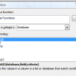
Database Functions include DSUM, DAVERAGE, DCOUNT. They are easy to use. You can use them with your Excel Tables and Lists. You use Database Functions to return the results (Sum, Average, Count, etc.) that you get from a Filter – or in this case, The Criteria.

Database Functions

Database Functions

Database Function Arguments

Each Database Function uses the same three required arguments:

  1.  
    1. Database. The Range that begins with your Data Set Labels and includes each column and each row in the database range. I prefer to use a “Named Range” for this argument.
  2. Field. The reference to the Field Label for the field that you wish to calculate (Sum, Count, Average, etc.) There are three ways to refer to this label: (Click on the cell with the label, use a column reference number (1,2,3, etc.) counting from Left to Right, type the “Label Name” inside ” ” quotation marks.
  3. Criteria. The Criteria Range that includes the Column Label for the criteria and the cells that contain the values or formulas you are using as your criteria.

It takes only a few minutes to set up your “Excel Dashboard” for the Criteria Range and your Results (e.g., the sum of the values in the field that match your criteria.) Change a value in your criteria and your results update automatically.

Filtering Data in Excel

If you use a structured data set in Excel, you probably use AutoFilters or Advanced Filters. Use Database Functions to “capture” the totals, averages, and counts of those queries.

If you need to review or learn how to apply Filters to data in Excel, watch these two lessons:

Click here to watch this video in High Definition at DannyRocksExcels on YouTube.

I invite you to shop for my DVD-ROM, “The 50 Best Tips for Excel 2007.” Click here to open a secure shopping cart.

Learn how to “Master Excel in Minutes – Not Months!”

Share and Enjoy:
  • Add to favorites
  • Facebook
  • Twitter
  • Technorati
  • Print
  • email
  • Digg
  • StumbleUpon
  • del.icio.us
  • Yahoo! Buzz
  • Google Bookmarks
  • Orkut
  • SphereIt
  • Sphinn

Working with Multiple Worksheets in Excel

The 50 Best Tips

The 50 Best

In this video lesson, I share my tips for maintaining a consistent look when working with multiple worksheets in Excel. I will demonstrate how to:

  • Group multiple worksheets for editing
  • Make a copy of an Excel worksheet
  • Use the Fill Across Worksheet tool – to update Contents or Formats or Both – for a Group of worksheets

In a professional setting, it is important to make a consistent presentation of your Excel worksheets. You want each worksheet in the group to use the same formatting styles, headers and formulas. The tips that I demonstrate will definitely save you time and help you to maintain a consistent look.

Click here to watch this video in High Definition, Full Screen mode on my DannyRocksExcels YouTube Channel.

Learn how to “Master Excel in Minutes – Not Months!”

Invitation to Visit My New Secure Online Shopping Site

I have just opened my new, secure online shopping website. I invite you to visit http://shop.thecompanyrocks.com to see the new products that I have introduced in the year 2011.

Share and Enjoy:
  • Add to favorites
  • Facebook
  • Twitter
  • Technorati
  • Print
  • email
  • Digg
  • StumbleUpon
  • del.icio.us
  • Yahoo! Buzz
  • Google Bookmarks
  • Orkut
  • SphereIt
  • Sphinn

Learn How to Use Date Functions in Excel

Excel has a group of functions that help you to calculate dates. For example, the number of days between two dates or the date on which an invoice will be payable.

This is the second in my series of lessons where I demonstrate how to enter and calculate dates and times in Excel. Here is the link to part one.

Excel Tip List

Excel DVD Tips

The date functions that I demonstrate on this video are:

  • TODAY()
  • NOW()
  • DATE()
  • DATEVALUE()
  • WORKDAY()
  • NETWORKDAYS()
  • EOMONTH()

The last three date functions require you to activate the Analysis ToolPak Add-in. You will also learn some valuable and time saving keyboard shortcuts.

You can watch this video in High Definition, Full Screen Mode on my YouTube Channel – DannyRocksExcels

Learn how to “Master Excel in Minutes – Not Months!”

Share and Enjoy:
  • Add to favorites
  • Facebook
  • Twitter
  • Technorati
  • Print
  • email
  • Digg
  • StumbleUpon
  • del.icio.us
  • Yahoo! Buzz
  • Google Bookmarks
  • Orkut
  • SphereIt
  • Sphinn

Use the SUMPRODUCT Function to Total Lists Using Multiple Criteria

In Excel 2007 and Excel 2010 you can use the new SUMIFS Function to total a list using multiple criteria. This is a great new feature!

But … what if you are using Excel 2003 or earlier? Or, if you collaborate with colleagues and clients who use older versions of Excel – how can you use multiple criteria to select the records that you want to Sum? You can use the SUMPRODUCT Function as I demonstrate in this video lesson.

The 50 Best Tips

The 50 Best Tips Series

Key Concepts

  • Create – and use – Named Cell References for Ranges / Arrays in your formulas
  • Use the Function Arguments Dialog Box – Use the keyboard shortcut Ctrl + A to bring this up
  • Use the F3 Keyboard Shortcut to bring up the Named Ranges List
  • In this lesson, use () to enclose each Array Argument
  • In this lesson, use * to substitute for the , to separate each Array in the formula (Edit this in the Formula Bar)

There are usually several ways to solve any problem in Excel. This is a good procedure to learn – regardless of the version of Excel that you use.

Click here to view the 1st part of this series on how to use the SUMPRODUCT Function in Excel.

You can view this Excel Video in Hig Definition, Full Screen Mode on my YouTube Channel – DannyRocksExcels by clicking here.

I cover the SUMIF and SUMIFS Functions in greater detail on my DVD, “The 50 Best Tips for Excel 2007.” Click here to start shopping using my secure shopping cart.

Learn how to “Master Excel in Minutes – Not Months!”

Share and Enjoy:
  • Add to favorites
  • Facebook
  • Twitter
  • Technorati
  • Print
  • email
  • Digg
  • StumbleUpon
  • del.icio.us
  • Yahoo! Buzz
  • Google Bookmarks
  • Orkut
  • SphereIt
  • Sphinn

How to Use the SUMPRODUCT Function in Excel

In my experience, most Excel users are unfamiliar with the SUMPRODUCT Function. So let me give you two reasons to watch this short (5 minutes, 22 seconds) video lesson to learn how – any why – to use SUMPRODUCT:

  1. The SUMPRODUCT Function will speed up your calculations in Excel – get results with one step. With SUMPRODUCT() you can avoid several intermediary calculations.
  2. With SUMPRODUCT, you may be able to trim the size of your Excel worksheet. You may not need as many columns (fields) as you think to get the result that you need!

In this lesson, I show you how to calculate the Total Value of the Inventory (for a fictional company) with one formula!

50 Best Tips for Excel 2007

Excel Tips

Key Points Coverered

While the SUM Function “Adds Up” the values in the Arguments, the PRODUCT Function “Multiplies” the values in its Arguments.

  • Using “Arrays” in SUMPRODUCTS. In Excel 2007, you can use up to 255 Arrays! The key point is that all Arrays must be the same size and shape. For example, if the 1st arry in the Arguments is 15 rows in one vertical column, then all of the subsequent Arrays must be 15 rows in one vertical column.
  • I find that Creating – and Using – Names Cell Ranges for the Arrays will speed up writing the SUMPRODUCT formula.

I have decided to present the SUMPRODUCT Function in two lessons – so click on the sequel to see other uses for this function!

Click here to watch the 2nd video lesson on how to use the SUMPRODUCT Function in Excel.

You can watch this Excel Training Video Lesson in High Definition, Full Screen Mode on my YouTube Channel – DannyRocksExcels

You can learn how to “Master Excel in Minutes – Not Months!”

Share and Enjoy:
  • Add to favorites
  • Facebook
  • Twitter
  • Technorati
  • Print
  • email
  • Digg
  • StumbleUpon
  • del.icio.us
  • Yahoo! Buzz
  • Google Bookmarks
  • Orkut
  • SphereIt
  • Sphinn