How to Take Advantage of Excel 2007 – 2010 Tables and Excel 2003 Lists

Excel Table Styles

Excel Table Styles

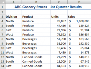
In this video tutorial, I cover multiple versions of Excel. I demonstrate how to take advantage of the Table Tools that were introduced in Excel 2007 and I also show you how to create Excel 2003 Lists.

Topics Covered on Video Tutorial

  • Convert a range of data to an Excel 2007, Excel 2010 Table.
  • Convert a range of data to an Excel 2003 List.
  • View and change the Total Row in each version of Excel.
  • Append new records to Tables and Lists.
  • Add a new field to Tables and Lists.
  • Write a formula in one cell of an Excel Table and have it automatically copy down for each record.
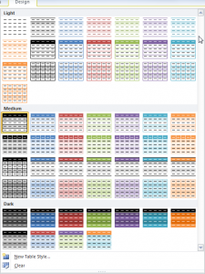
  • Change the Table Styles in Excel 2007 and 2010.
  • Use Conditional Formatting to add alternate row shading to an Excel 2003 List

Watch Video in High Definition on YouTube

Follow this link to watch this Excel Video Tutorial in High Definition on my YouTube Channel, DannyRocksExcels

Download This Excel Workbook

Click on this link to download the Excel Workbook that I used in this video tutorial.

Get my best-selling DVD-ROM, “The 50 Best Tips for Excel 2007” for only $39.95!
Share and Enjoy:
  • Add to favorites
  • Facebook
  • Twitter
  • Technorati
  • Print
  • email
  • Digg
  • StumbleUpon
  • del.icio.us
  • Yahoo! Buzz
  • Google Bookmarks
  • Orkut
  • SphereIt
  • Sphinn

Dynamically Update a Cell with an Excel Worksheet Name

Formula to Capture Worksheet Name

Capture Tab Name in Cell

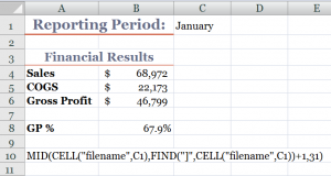
I am excited to share this Excel Tip with you! Several viewers have recently asked if there was a way to create a link in a cell to the name of a worksheet tab. Yes there is! And, in this lesson, I demonstrate how to do this.

Say, for example, that you want Cell C1 to contain the name of the current worksheet (Sheet1). With this formula, when you change the name of the worksheet to “January,” cell C1 is dynamically updated to show “January.”

Perfect for Excel Templates

If you use a template for your monthly, regional sales or financial reports, then this Excel formula is essential. You write the formula once – using Group edit – and each worksheet in your Excel workbook will be linked to a cell in your report. Change the name of the worksheet and your report name is automatically updated.

Functions Used in this Formula

  • CELL() – to gather information about the worksheet – in this case, the “Filename.”
  • MID() – to extract the characters in a text string – e,g, the “worksheet name.”
  • FIND() – to locate the starting point for the MID() function to extract the characters in the text.

As the final argument for the MID() Function, I use 31 characters because that is the maximum number of characters that you can use when naming an Excel worksheet.

Try this for yourself. Let me know how it works for you. Add your comments below.

Download Excel Workbook for this Lesson

Watch Video in High Definition

Follow this link to view this video tutorial on my YouTube Channel – DannyRocksExcels

I invite you to watch or to subscribe to my video podcast on iTunes. Follow this link to learn more about my RSS Feed.

Share and Enjoy:
  • Add to favorites
  • Facebook
  • Twitter
  • Technorati
  • Print
  • email
  • Digg
  • StumbleUpon
  • del.icio.us
  • Yahoo! Buzz
  • Google Bookmarks
  • Orkut
  • SphereIt
  • Sphinn

How to Search For and Use Text Strings in Excel

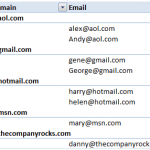
A viewer asked for my help in creating a report that will group his customers’ email addresses by their “domain name.” For example, he wants to be group all customers with gmail addresses . Likewise, his  customers’ yahoo mail, aol.com accounts, etc.

Pivot Table for Email Domains

Pivot Table Email Domains

I immediately decided to use two powerful Excel tools to produce this report:

  1. Text-to-Columns to create two columns (name and domain) from one text value (the email address).
  2. Pivot Table Report to group and present customer emails by domain name.

Both tools work great and I produced the report with only a few mouse clicks!

The response that I got from my viewer was, “That’s great Danny. But …”

It turns out that the viewer wanted to have the Domain Names as the Field Headers and to show each customer’s email address as a row going down vertically in the corresponding field. To give my viewer the report that he wanted, I used these tools and techniques:

  • I returned to the Pivot Table to copy the unique list of domain names.
  • I used Paste Special – Transpose to convert the vertical list of domain names into a horizontal row of Field Headers.
  • I began to build my “Mega-formula” by taking “baby steps” – i.e. I created one formula and then “nested” it inside additional formulas and functions.
  • For the first “baby step” formula I used the SEARCH() Function.
  • Next, I “nested” this formula as the “logical test” inside an IF() Function.
  • In order to “hide” all of the formula error signs, I nested both of these functions inside the NEW IFERROR() Function.
  • IFERROR() was introduced in Excel 2007 and I now consider it to be “indispensable!” This function, alone, makes upgrading to either Excel 2007 or Excel 2010 a “nobrainer” decision!

I enjoy answering questions from my viewers. Many of these questions can be answered from one of the lessons on my DVD-ROM, “The 50 Best Tips for Excel 2007.” For the rest, I try to create a video lesson that demonstrates how to get the answers that you – my viewers and customers – are looking for.

Keep your questions and suggestions coming! I enjoy receiving feedback from you!

I invite you to subscribe to my RSS Feed on Feedburner to be automatically notified whenever I publish a new Excel Video Tutorial.

Watch this Excel Video in High Definition on YouTube

Here is the link to watch this video on my YouTube Channel – DannyRocksExcels

Share and Enjoy:
  • Add to favorites
  • Facebook
  • Twitter
  • Technorati
  • Print
  • email
  • Digg
  • StumbleUpon
  • del.icio.us
  • Yahoo! Buzz
  • Google Bookmarks
  • Orkut
  • SphereIt
  • Sphinn

Use SumIf and SumIfs Function in Accounts Receivable Status Report

I receive many requests from viewers to help them to create and to analyze “Accounts Receivable Reports.” So, I created this Excel Video tutorial to demonstrate how both the SUMIF and the SUMIFS Functions can help you to analyze the data in an AR Status Report.

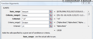
The SUMIF() Function has been available for many years in Excel – and it is a great function to use. However, starting in Excel 2007, we now have the expanded SUMIFS Function which allows us to evaluate multiple ranges using multiple criteria to return the sum of our results. This is a terrific improvement!

SUMIFS Function

SUMIFS in Excel 2007

Use SUMIFS() Function

With the SUMIFS Function, you no longer have to create multiple, complicated “nested IF Functions. Rather. you use a series of “paired arguments” – Criteria Range1, Criteria1″ etc. to define the result that you want to return.

So, with the SUMIFS() Function, you can use “paired” Criteria Ranges and Criteria to produce the exact results that you are seeking!

This, alone, may be one of the reasons to upgrade to either Excel 2007 or to Excel 2010!

Watch this Video in High Definition mode on YouTube

Here is the link to view this Excel lesson in High Definition on my YouTube Channel

You can learn how to “Master Excel in Minutes – Not Months!”

Share and Enjoy:
  • Add to favorites
  • Facebook
  • Twitter
  • Technorati
  • Print
  • email
  • Digg
  • StumbleUpon
  • del.icio.us
  • Yahoo! Buzz
  • Google Bookmarks
  • Orkut
  • SphereIt
  • Sphinn

How to Use the Average Functions in Excel 2007 and 2010

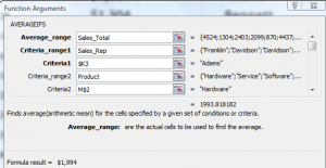
The new AVERAGEIF and AVERAGIFS Functions were introduced in Excel 2007. In this lesson, I demonstrate how and when to use both functions. If you are using an earlier version of Excel – e.g. Excel 2003, I show you how to use a Pivot Table to produce the same results.

Average is not the Median

The Average Function is the “Arithmetic Mean” of the range of cell values. This means the Sum of the values in the range divided by the Count of the cells with numeric values in the range. Many people confuse this with the MEDIAN sale which is the “middle value” in the range. Half of the cell values are above and half of the cell values are below the result of the MEDIAN() Function.

New AverageIfs Function in Excel

AverageIfs Function

New Functions in Excel 2007

Watch the video to see how to use both the AverageIf and AverageIfs Functions. I recommend using the Function Arguments Dialog Box and Named Cell References with these functions. Pay attention to my use of “Mixed Cell References” in the AverageIfs formula. Doing so makes it easy to write the formula in one cell and then copy it across the range of cells.

Here is the link to watch this video tutorial in High Definition on my YouTube Channel.

Learn how you can “Master Excel in Minutes – Not Months!”

Share and Enjoy:
  • Add to favorites
  • Facebook
  • Twitter
  • Technorati
  • Print
  • email
  • Digg
  • StumbleUpon
  • del.icio.us
  • Yahoo! Buzz
  • Google Bookmarks
  • Orkut
  • SphereIt
  • Sphinn

How to Find and Delete Duplicate Records in Excel 2007

It is easy  – much too easy – to allow duplicate records to creep into an Excel database. Fortunately, starting in Excel 2007, it is really easy to first find and then delete duplicate records.

Remove DUplicate Records

Remove Duplicate Records

With the price of postage climbing, you cannot afford to send duplicate copies of a mailing piece. Not to mention that doing so reflects poorly on your company’s organizational skills. Likewise, having duplicate account entries makes for extra work and confusion.

Use Conditional Formatting to Highlight Duplicate Records

Starting in Excel 2007, Conditional Formatting got a lot easier to use. One of the menu selections is “Show Duplicate Records.” Now, with just a few mouse clicks, you can format the records that show duplicate values in your data set. I like to use this technique prior to acutally duplicating records so that I can get a sense of the number of possible duplicate records in my data set.

Selecting Duplicate Records to Delete

As a best practice, I always make a backup copy of my data set before I actually delete records. This way, I can quickly recover from any accidental deletions of non-duplicate records. When you choose the command to “Remove Duplicates,” a dialog box opens to reveal each field in your data set. Generally, you want to select all of the fields to narrow down the list of records to delete. Since I have already previewed the possible duplicate records by using Conditional Formatting, I have a pretty good idea of how many records will be deleted. You do not see a preview of the exact records that will be deleted, so make sure that you have a backup copy of your original list in order to restore any “accidental” deletions.

These new commands and menus introduced in Excel 2007 make deleting duplicate records a very quick process. Use them – wisely – to save yourself time, confusion and money!

Learn how to “Master Excel in Minutes – Not Months”

Watch this video lesson in High Definition, Full Screen mode. Follow this link to view this on my YouTube Channel – DannyRocksExcels

Secure Shopping Cart

Secure Shopping Cart

This is one of the tips that I offer on my DVD, “The 50 Best Tips for Excel 2007.” CLick here to open a secure shopping cart to purchase it.

Share and Enjoy:
  • Add to favorites
  • Facebook
  • Twitter
  • Technorati
  • Print
  • email
  • Digg
  • StumbleUpon
  • del.icio.us
  • Yahoo! Buzz
  • Google Bookmarks
  • Orkut
  • SphereIt
  • Sphinn

Learn How to Quickly Create Excel Pivot Table Reports

Excel Data Set

Data Set in Excel

Many people are curious about Excel Pivot Tables. They would like to learn how to create a Pivot Table, but they fear that that will take too long and be difficult to learn. 

Here’s the good news! Pivot Tables are one of the most powerful tool in Excel AND Pivot Tables are also one of the easiest Excel Techniques to learn! It sounds like a contradiction, doesn’t it? 

How would you like to turn this data set – with over 500 rows of data … 

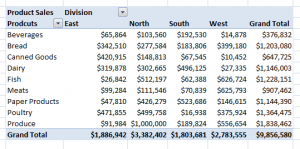
into this Pivot Table Summary Report with @ six clicks of the mouse? 

Pivot Table Row & Column

Pivot Table Summary

 That’s all it takes. With a Pivot Table you turn long lists of data into summarized information that highlights the trends and patterns in your business. 

Special: Save 20% on any purchase! Use Coupon SAVE-20-PCT during Checkout! 

I can teach you how to get started on the road to mastering Excel Pivot Tables. On my DVD-ROM, “The 50 Best Tips for Excel 2007,” I have the following Pivot Table video lessons: 

  • Introducing Pivot Tables – Run time: 8:23
    • Why Use Pivot Tables?
    • How to Create a Pivot Table
    • How to Modify a Pivot Table
    • How to Update a Pivot Table
  • Grouping and Charting in Pivot Tables – Run time: 5:50
    • Grouping Pivot Table Fields by Month, Quarter and Year
    • Grouping Pivot Table Fields by Week
    • Collapsing and Expanding Pivot Table Fields
    • Creating Pivot Charts
  • Using New Pivot Table Features in Excel 2007 – Run time: 7:46
    • Base Your Pivot Table on an Excel Table
    • Adjust Pivot Table Report Layouts
    • Apply Conditional Formatting to Pivot Tables
    • Insert Blank Rows in Your Pivot Table Report
The 50 Best Tips

The 50 Best Tips Series

As you can see from the “Run times,” each lesson is focused on one Excel technique. If you don’t have a lot of time and you want to quickly learn how to create Pivot Tables, my DVD-ROM is the best place to begin. 

Here is a PDF that you can download to see the content and Run times for each of my tips: The 50 Best Tips for Excel 2007 Detailed Content Listing 

And, here is a link to my Archive of Free Pivot Table Videos  on The Company Rocks website. 

Learn how to “Quickly Create Excel Pivot Table Reports and Charts” 

Thank you! 

Danny Rocks

Share and Enjoy:
  • Add to favorites
  • Facebook
  • Twitter
  • Technorati
  • Print
  • email
  • Digg
  • StumbleUpon
  • del.icio.us
  • Yahoo! Buzz
  • Google Bookmarks
  • Orkut
  • SphereIt
  • Sphinn

Using the Built-in Excel Data Form to Edit, Enter and View Records

Data Form in Excel

Data Form

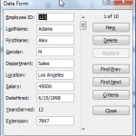
Excel has a built-in Data Form which is very useful for viewing all of the fields (up to 32 of them) associated with a single record. When you have lots of “Fields” in your “Data Set” and you do not want to do a lot of horizontal scrolling to view or edit the values in the cells, use this Data Form.

There is a limit of 32 fields when using Excel’s built-in Data Form.

Customize the Quick Access Toolbar

However, it does not appear as a Ribbon Command in Excel 2007. To use the Data Form add the Form Command to your Quick Access Toolbar (QAT) – I show you how to do this in the video.

Personally, I do not recommend the Excel Data Form for entering new records in your data set. I like to add Data Validation drop-down lists to ensure data integrity and this feature is not available in the Data Form. However, you can use Criteria to quickly find records for viewing and editing in the form.

Filtering Data with the Data Form

I give you a brief introduction to some of the new filtering options available in Excel 2007. I will cover this in greater detail in another lesson.

Subscribe to My Video Podcast on iTunes

I invite you to subscribe to my free video podcast, “Danny Rocks Tips and Timesavers” on iTunes. Click here to go directly to my iTunes podcast. I have had over 25,000 downloads since I began my podcast in June of 2010.

Watch this video in High Definition

Click here to go to my DannyRocksExcels YouTube Channel.

Watch Video Now

Master Excel in Minutes Video Training Resources

I have created a series of extended length Excel Video Training Resources. I invite you to visit my secure online shopping site to: Learn how to “Master Excel in Minutes – Not Months!”

Share and Enjoy:
  • Add to favorites
  • Facebook
  • Twitter
  • Technorati
  • Print
  • email
  • Digg
  • StumbleUpon
  • del.icio.us
  • Yahoo! Buzz
  • Google Bookmarks
  • Orkut
  • SphereIt
  • Sphinn

My Most Viewed and Downloaded Videos for Excel and PowerPoint

My iTunes Podcast

Danny on iTunes

I began to post my videos as podcasts at the iTunes store this past summer. Since then, my video lessons for Excel and PowerPoint have been viewed and downloaded many times. I am thirlled. And, I thank you for your support and encouragement.

Here are the links – on my website – to the most popular video episodes. I have organized them by category in the order of their popularity. You can click on any link to view or download that video from my website. Or, you can go to my video Podcast by clicking on this link – “Danny Rocks Tips and Timesavers” Podcast on iTunes.

Merging and Consolidating Excel Worksheets

 PowerPoint Presentations

Data Visualizations

What-If Analysis in Excel

Importing Data From Other Programs

Pivot Tables

Excel Tables

Social Media

Formula Errors

Please add your comments below – or on my iTunes Channel. I welcome your feedback.

You can learn how to “Master Excel in Minutes – Not Months!”

Sincerely,

Danny Rocks

Share and Enjoy:
  • Add to favorites
  • Facebook
  • Twitter
  • Technorati
  • Print
  • email
  • Digg
  • StumbleUpon
  • del.icio.us
  • Yahoo! Buzz
  • Google Bookmarks
  • Orkut
  • SphereIt
  • Sphinn

Five Benefits from Using Tables in Excel 2007

I really enjoy the major changes that Excel 2007 has incorporated into Tables. In this video I demonstrate Five Benefits when you convert your Excel data lists into Tables.

(Note: This is a re-post. I now make many of my videos available as Podcasts and I need to send these videos to the iTunes store.)

Click here if you would like to subscribe to my Podcast at the iTunes store.

Learn how to “Master Excel in Minutes – Not Months!”

Share and Enjoy:
  • Add to favorites
  • Facebook
  • Twitter
  • Technorati
  • Print
  • email
  • Digg
  • StumbleUpon
  • del.icio.us
  • Yahoo! Buzz
  • Google Bookmarks
  • Orkut
  • SphereIt
  • Sphinn