Pivot Tables | The Company Rocks

Danny April 19, 2011 Leave a Comment

Download My Excel Workbooks and Step-by-Step Instructional Manuals for Free!

Finally! I have figured out a way to allow my viewers to download the Excel Workbooks, Word Documents, PowerPoint Presentations, etc. that I use in my video lessons. For the past few months, I have been able to give you a direct link to download the Adobe Acrobat files that I create. For example:

My problem has been that – Starting in Office 2007 – the underlying file structure of each program (Excel, Word, PowerPoint, etc.) has changed and it is no longer possible to “Publish to the Web” the worksheets, documents and presentations that I offered in the past. I will spare you the boring details of why and how this has happened, because I have good news for you!

Enter, “The Cloud!”

Cloud Computing

You have probably seen or heard this advertising slogan recently. Here is how I have just discovered how “The Cloud” can work for both you and me:

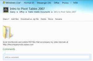
I have created a Danny Rocks “Sky Drive” folder where I can post – and you can download – the Workbooks, Documents and Presentations that I create and choose to share!

Initially, I am uploading – and sharing – the workbooks, documents, PDFs, etc. that accompany the extended video recordings that I offer on my http://thecompanyrocks.webex.com site.

This is a new development for me and The Company Rocks. I offer a series of extended length ( 25 minute to 60 minutes) video tutorials.

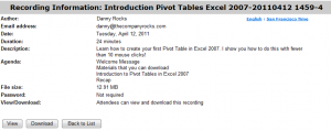
Information about this Video Recording
As I write this posting, I have 4 modules – each offered “free of charge” – for you to view and / or download.

Go to http://thecompanyrocks.webex.com to see what I currently offer you!

As I gather feedback, activity, statistics, etc. I may extend the range of downloadable content that I create – My decision will depend upon your feedback, so please add your comments below in this posting!

My Next Level of Product Offerings

I am on a journey to evolve the range and detail of the products and services that I offer you, my loyal viewers and subscribers. I wnat to be responsive to your needs. So, that meanrs that the more feedback that I get from you – my viewers and subscribers – the better I can structure my offerings. I welcome your feedback!

Based on some great feedback from my viewers and subscribers, I have just begun to create a series of extended length ( 25 to 45 minutes) video tutorials. The initial tutorials will be offered “free of charge.” Other video tutorials will be carry a modest – I might add, aggressive – pricing model! My goal is to give you the product and content that you need at a price that is mutually acceptable! You, and your level of supposrt will tell me what is acceptable – please give me your feedback!

Extended Video Tutorials Now Online

You can now view or download – after registering – at WebEx by Cisco – for these video tutorials that I have posted:

Introduction to Pivot Tables in:
- Excel 2007
- Excel 2003
Merge Mailing Labels in:
- Office 2007
- Office 2003

I hope that you find these links and videos helpful. Please add your feeback via the comments section below this post.

Sincerely,

Danny Rocks

www.thecompanyrocks.com

Share and Enjoy:

Filed Under: Download Files from Video Lessons, Excel Training, Integrating MS Office Programs, Pivot Tables, WebEx by Cisco, WebEx Recordings & Webinars Tagged: Download Excel Workbooks, Excel Video Training, Merge Mailing Labels in Office 2003, Merge Mailing Labels in Office 2007, Merging Mailing Labels in Word, Pivot Table Drop Areas, Video lessons for Excel

Danny April 13, 2011 Leave a Comment

Announcing My Online Courses – Master Business Skills in Minutes

I am proud to announce that I have posted the first two recorded video lessons for my online course: “Master Excel in Minutes!”

WebEx Navigation Pane

These courses are recorded in-depth videos that you can choose to watch online or download to your computer to watch at a later time. Some of the recordings will be offered free of charge. For others – which contain premium content – I will charge a fee. The recorded videos will be found on my website at WebEx:

http://thecompanyrocks.webex.com

New Page on My Website

You can find more information about my online courses by following this link to a new page that I have created here on my website.

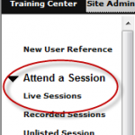
Here are the direct links to my first two recorded video lessons on WebEx – be sure to click the “Recorded Sessions” on the main “Attend a Session” navigation pane at http://thecompanyrocks.webex.com:

Introduction to Pivot Tables in Excel 2007 – Run time: 24 minutes Fee: Offered free of charge (after registration).
Introduction to Pivot Tables in Excel 2003 – Run time: 28 minutes Fee: Offered free of charge (after registration).

In this format – recorded, downloadable, video lessons – I am able to go into more detail on the topic than I do with my free video podcasts. I can also cover – in depth – topics that my viewers have been requesting. For example, I can now train you in MS Office 2003 (Excel 2003, Word2003, etc.)

Contents of Recorded Video Lessons

Each of the recorded video lessons includes:

The recorded video lesson that you can watch online
The recorded video lesson that you can download to your computer to view at a later time
The workbooks or documents that I use during the lesson – so that you can practice the concepts that I present on the video recording.
A PDF containing the Step-by-step instructions for each lesson – so that you can make notes as you view the recording or during your practice sessions.

I hope that you will take a few minutes to view my first offerings in this course. After you watch the lessons, please send me your feedback, questions and suggestions for future course offerings.

Thank you!

Danny Rocks

Share and Enjoy:

Filed Under: Business Practices, Excel Training, Pivot Tables, WebEx Recordings & Webinars Tagged: Excel Pivot Tables, Excel Video Training, Video lessons for Excel

Danny April 3, 2011 Leave a Comment

How to Search For and Use Text Strings in Excel

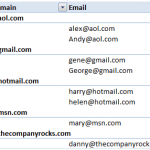
A viewer asked for my help in creating a report that will group his customers’ email addresses by their “domain name.” For example, he wants to be group all customers with gmail addresses . Likewise, his customers’ yahoo mail, aol.com accounts, etc.

Pivot Table Email Domains

I immediately decided to use two powerful Excel tools to produce this report:

Text-to-Columns to create two columns (name and domain) from one text value (the email address).
Pivot Table Report to group and present customer emails by domain name.

Both tools work great and I produced the report with only a few mouse clicks!

The response that I got from my viewer was, “That’s great Danny. But …”

It turns out that the viewer wanted to have the Domain Names as the Field Headers and to show each customer’s email address as a row going down vertically in the corresponding field. To give my viewer the report that he wanted, I used these tools and techniques:

I returned to the Pivot Table to copy the unique list of domain names.
I used Paste Special – Transpose to convert the vertical list of domain names into a horizontal row of Field Headers.
I began to build my “Mega-formula” by taking “baby steps” – i.e. I created one formula and then “nested” it inside additional formulas and functions.
For the first “baby step” formula I used the SEARCH() Function.
Next, I “nested” this formula as the “logical test” inside an IF() Function.
In order to “hide” all of the formula error signs, I nested both of these functions inside the NEW IFERROR() Function.
IFERROR() was introduced in Excel 2007 and I now consider it to be “indispensable!” This function, alone, makes upgrading to either Excel 2007 or Excel 2010 a “nobrainer” decision!

I enjoy answering questions from my viewers. Many of these questions can be answered from one of the lessons on my DVD-ROM, “The 50 Best Tips for Excel 2007.” For the rest, I try to create a video lesson that demonstrates how to get the answers that you – my viewers and customers – are looking for.

Keep your questions and suggestions coming! I enjoy receiving feedback from you!

I invite you to subscribe to my RSS Feed on Feedburner to be automatically notified whenever I publish a new Excel Video Tutorial.

Watch this Excel Video in High Definition on YouTube

Here is the link to watch this video on my YouTube Channel – DannyRocksExcels

Share and Enjoy:

Searching for Text Strings in Excel [ 9:36 ] Play Now | Play in Popup | Download (1139)

Filed Under: Excel Training, New in Excel 2007, Pivot Tables, Podcast Tips & Timesavers, Text Functions Tagged: Excel Pivot Tables, Excel Video Training, If Functions in Excel, IF() Function, IFERROR Function, MegaFormulas, Mixed Cell Reference, Nesting Formulas and Functions, SEARCH() Function, Text Functions in Excel, Text-to-Columns Data Tool, Video lessons for Excel

Danny March 26, 2011 Leave a Comment

How to Take Advantage of Report Filters in Excel Pivot Tables

Starting with Excel 2007, Pivot Tables now include a “drop field” labeled “Report Filters.” The Report Filters area replaces the area labeled the “Pages” drop area in Excel 2003 and earlier. Report Filters is a more descriptive and intuitive name. So , this is a welcome change.

Use Report Filters in Pivot Table

In this lesson, I am responding to an additional request from one of my viewers who wants me to demonstrate how the “Report Filters” drop zone will provide incredible reporting power in a Pivot Table.

Request from a Viewer

In this lesson, my viewer is a “hydrologist” who analyzes average Water Flows by day and by month in a “Water Year.” If you use a “Fiscal Year” reporting structure, you will want to pay attention to this lesson. In this case, the “Water Year” begins on October 1 and ends on September 30. My viewer needs my help in separating out individual Pivot Table Reports organized by Water Year – placed in the Report Filters Drop Zone.The Pivot Tables show the average daily water flow by date. He told me that he is concrned that that Pivot Table Report may not be able to “account for Leap Years.”

Not to worry!

Watch this Excel Video Tutorial, as I demonstrate how to answer my viewer’s query and also give you some “solid tips” to get the results that you need when using Excel!

Watch this Excel Video Tutorial in HD Mode on my YouTube Channel

Here is the link to my YouTube video channel for this video.

Learn how to “Quickly Create Pivot Table Reports!”

Share and Enjoy:

Taking Advantage of Report Filters in Excel Pivot Tables [ 8:51 ] Play Now | Play in Popup | Download (959)

Filed Under: Excel Training, Pivot Tables, Podcast Tips & Timesavers Tagged: Choose Function in Excel, Create Fiscal Year Reports in Excel, Day Function in Excel, Excel Pivot Tables, Excel Video Training, MONTH Function, Pivot Table for Fiscal Year, Pivot Table for Water Year, Pivot Table Report Filters, Pivot Tavle Report Filters, Show Report Filter Pages, Video lessons for Excel, YEAR() Function

Danny March 11, 2011 Leave a Comment

How to Generate Multiple Reports from One Pivot Table

You can create an Excel Pivot Table with just a few mouse clicks. And, with just a few more clicks, you can change – or pivot – the design of your report. Most people who use Pivot Tables know this. However, I find that most Excel users do not know that you can generate multiple reports – each one on a separate worksheet – with just a few clicks. This is a tremendous time-saving tip!

Multiple Reports

Pivot Table Report Filters

When you place one or more fields in the “Report Filters” drop zone of your Pivot Table, you will be able to generate multiple reports from one Pivot Table. Report Filters were introduced in Excel 2007. If you use an earlier version of Excel, this drop zone is called, “Pages.” Report Filters allow you to create interactive views of your data. If you use Dashboard Reports, you will want to include Report Filters in your Pivot Table.

In this video, I demonstrate how to generate reports – each on an individual worksheet – for the values in your Report Filter Field. Whenever I demonstrate this technique in a class or to a client, I always get a “gasp of excitement.” Most people say, “That’s incredible. Do that again!”

Create a Calculated Field

I also show you how to Create a Calculated Field in a Pivot Table. You do not need to return to your source data to add additional fields and then recreate your Pivot Table. Why keep redundant data? Rather, create as many Calculated Fields as you need in your Pivot Table.

Copy Your Pivot Table

You can prevent “Pivot Table Bloat” when you make copies of a Pivot Table rather than creating brand new Pivot Tables from the same source data. Watch as I demonstrate how to do this.

Follow this link to learn how you can “Quickly Create Pivot Tables and Charts”

Here is the link to watch this video in High Definition on my YouTube Channel, DannyRocksExcels

Share and Enjoy:

Generate Multiple Reports from One Pivot Table [ 8:26 ] Play Now | Play in Popup | Download (3693)

Filed Under: Excel Training, Pivot Tables, Podcast Tips & Timesavers Tagged: Calculated Fields in Pivot Tables, Copy a Pivot Table, Excel Pivot Tables, Excel Video Training, Pivot Table Report Filters, Show Report Filter Pages, Video lessons for Excel

Danny March 6, 2011 1 Comment

How to Sort Pivot Table Field Values in Excel

With a Pivot Table, you have more options and more flexibility when it comes to sorting your field values than you do with a regular Excel data set. However, many of my clients and viewers seem to get “lost” when it comes to creating custom sorts for their Pivot Table Field Valuess. So, let me demonstrate four ways to sort fields to suit your needs.

Sort Pivot Table Fields

Sort the Order of Months

If you create a Pivot Table for a Fiscal Year or,as in this example a Water Year, you will want to sort the Month Fields to match the starting and ending months in your FY. There are at least three ways to do this:

Right click on the month that you want as your first month. Choose Move from the shortcut menu and select Move (in this case) Oct to Beginning.
Another way to relocate a field value is to select the bottom part of the cell. When you see the 4-heard black cross, just move the field value to the new location. You will see a Gray Horizontal Bar as you drag the field.
Most amazing way to move a field value – and seeing is believing – is to go to the cell where you want to place the field value and just “type in the name of the field value. Incredibly, Excel moves the field values to accommodate the value that you typed in! This only works with a Pivot Table.

Sort Using a Custom List

You can create a Custom List and use that for sorting the values in your Pivot Table Field. After you create your Custom List (I show you how in this video) you choose the Pivot Table Options Sort command and then choose the direction – Ascending or Descending.

In Pivot Tables, Excel remembers your custom Field Value Settings when you move – or Pivot – field from Rows to Columns for example.

After you watch this short five minute video lesson you will know how to sort field values in Pivot Tables to suit your needs.

Pivot Table Resources

Pivot Table Training Resources

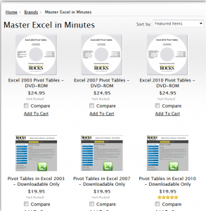
I have published 90 Minute Video Tutorials to help you to quickly master Pivot Tables. No matter which version of Excel that you are using (Excel 2010, 2007, or 2003), I offer video training that is specific to your version. You can learn more about these resources at my secure online shopping website – http://shop.thecompanyrocks.com

Learn how to “Quickly Create Pivot Tables and Charts”

My YouTube Channel – DannyRocksExcels

Click here to watch this video in High Definition, Full-screen mode

Share and Enjoy:

How to Sort Pivot Table Fields in Excel [ 5:01 ] Play Now | Play in Popup | Download (1124)

Filed Under: Excel Training, Pivot Tables, Podcast Tips & Timesavers Tagged: Excel Pivot Tables, Excel Video Training, Pivot Table for Water Year, Pivot Tables for Fiscal Year, Sort field vales by typing name, Sort Pivot Table Field Values, Sort using an Excel Custom List, Video lessons for Excel

Danny March 4, 2011 1 Comment

Create a Pivot Table for a Water or Hydrological Year

A viewer asked for my help in creating a Pivot Table Report that is based on a Water Year – also known as a Hydrological Year. In North America, a Water Year begins on October 1 and ends on September 30. If you use a Fiscal Year in your reporting, you will want to watch this Excel Training Video Lesson.

Pivot Table for Water Year

Add Two Fields to Source Data

In order for a Pivot Table to summarize non-calendar years and quarters you will need to have two additional fields in your source data:

A Fiscal Year (Water Year) Field – Use the IF(), MONTH() and YEAR() Functions to produce this.
A Fiscal Quarter (Hydrological) Quarter Field – Use the CHOOSE() Function to produce this.

Now you are ready to create your Pivot Table Report.

Group Dates by Month and Year

Begin by grouping the Date Field by Month and Year – not, in this case, by Quarter. Now, remove the new Year field that you just created and add in the Water Year Field and the Hydrological Quarter to the Pivot Table. Continue to arrange the Pivot Table to suit your needs.

Since there is no direct way to change a Calender Year into a Fiscal Year or Water Year, you must prepare your data prior to beginning to create your Pivot Table. Now that you have watched this video lesson, you know how to do this!

Learn how to “Quickly Create Excel Pivot Tables and Charts”

Create Dynamic Chart Titles in Excel

A viewer wrote to ask for my help in creating dynamic chart titles in Excel. He has created a series of pivot table reports and pivot charts. He wants the titles for his charts to update dynamically. That is, as he selects a new filter for his pivot table, he wants the title in his pivot chart to match the value label in his filter.

: Dynamic Chart Titles

Note:

This technique will work for all Excel Charts and Chart Types. It is not restricted to Pivot Tables.

The solution is rather simple: You link the Chart Title to a formula.

Link Chart Title to Formula

Select a cell that is outside the range of your Pivot Table – let’s say cell H1. An example formula is:

=”Sales for Fiscal Year “&D1

In this case, cell D1 contains the label for the value that you are selecting to filter your Pivot Table Report and Chart – e.g. 2008 as your Fiscal Year.

Notice that in the formula, I include the “TEXT” inside ” ” (double quotation marks. I also use the & (ampersand) to join the text to the cell reference (D1).

Finally, select the Chart Title and then, in the formula bar type =H1 (where H1 is the cell that contains the formula that we just wrote).

As a finishing touch, you can “hide” the formula in cell H1 by changing the FONT COLOR to match the background color for that cell.

It is that easy! Try it yourself after you watch this short (6 minutes) video lesson.

Invitation to Visit My New Online Shopping Site

Shop for The 50 Best Tips for Excel 2007

My new, secure, online shopping website – http://shop.thecompanyrocks.com – is now open. I invite you to stop by for a visit and get more information about the many resources that I offer for sale including, “Learn how to “Master Excel in Minutes – Not Months!”

Watch Tutorial in High Definition

Follow this link to my YouTube Channel – DannyRocksExcels – where you can watch this video lesson in High Definition, Full-screen mode.

Share and Enjoy:

Creating Dynamic Chart Titles in Excel [ 6:09 ] Play Now | Play in Popup | Download (2578)

Filed Under: Excel Charts, Excel Formulas, Excel Training, Pivot Tables, Podcast Tips & Timesavers Tagged: Chart Titles, Excel Charts, Excel Pivot Tables, Excel Video Training, Pivot Charts, Pivot Table Report Filters, Update Chart Titles, Video lessons for Excel

Danny January 1, 2011 Leave a Comment

The 10 Most Watched Videos at The Company Rocks During 2010

Reminder Note

I like to look back to review the results of the past year. Which posts, which videos were the most popular, which videos were downloaded most often? As I look at this list of 10 videos, the clear winner – by category – is merging data from multiple worksheets. Three of the top 10 videos that were watch the most fall into this category!

Here is a listing of the 10 Video Lessons that were watched most frequently on my website – www.thecompanyrocks.com – during 2010:

1- Summarize Multiple Excel Worksheets – Consolidate by Position

2- Build an Accounts Receivable Aging Report

3- Use Pivot Tables to Summarize by Year, Quarter and Month

4- Simplify Data Lookups in Excel

5- Perform Break-Even Analysis with Excel’s Goal Seek Tool

6- How to Display Numbers During a PowerPoint Presentation

7- Make Excel Data Come Alive with Visualization Tools

8- Excel 2003 Basics – Data Entry

9- How to Merge Multiple Excel Workbooks into a Master Budget

10- Consolidate Data from Multiple Excel Worksheets – Part 2 – by Category

If you enjoy these videos, you will enjoy my DVD-ROMs, “The 50 Best Tips for Excel 2007” and “The 50 Best Tips for PowerPoint 2007.” You can use my secure shopping cart to purchase them now.

I have reduced the purchase price of my Individual DVD-ROMs to $29.97 USD. You do not need a coupon to receive this special price. Simply, go to my online store – http://shop.thecompanyrocks.com

You can also watch my videos on iTunes. Click here to go to my Video Podcast, “Danny Rocks Tips and Timesavers” at the iTunes Store.

Learn how to “Master Excel in Minutes – Not Months!”

My most recent videos can be viewed in High Definition, Full Screen Mode on my YouTube Channel – DannyRocksExcels

Share and Enjoy:

Filed Under: Consolidate Excel Data, Excel Basics, Excel Financial Tools, Excel Training, Goal Seek in Excel, Lookup Functions in Excel, Most Viewed Excel Videos, Pivot Tables, Powerpoint Techniques Tagged: Consolidate Excel data, Excel Pivot Tables, Excel Video Training, Group Dates in Pivot Tables, Lookup Functions in Excel, Most Viewed Excel Videos, PowerPoint Presentations, Tips and Time Savers, Video lessons for Excel

Danny December 20, 2010 1 Comment

Learn How to Quickly Create Excel Pivot Table Reports

Data Set in Excel

Many people are curious about Excel Pivot Tables. They would like to learn how to create a Pivot Table, but they fear that that will take too long and be difficult to learn.

Here’s the good news! Pivot Tables are one of the most powerful tool in Excel AND Pivot Tables are also one of the easiest Excel Techniques to learn! It sounds like a contradiction, doesn’t it?

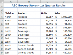
How would you like to turn this data set – with over 500 rows of data …

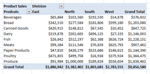
into this Pivot Table Summary Report with @ six clicks of the mouse?

Pivot Table Summary

That’s all it takes. With a Pivot Table you turn long lists of data into summarized information that highlights the trends and patterns in your business.

Special: Save 20% on any purchase! Use Coupon SAVE-20-PCT during Checkout!

I can teach you how to get started on the road to mastering Excel Pivot Tables. On my DVD-ROM, “The 50 Best Tips for Excel 2007,” I have the following Pivot Table video lessons:

Introducing Pivot Tables – Run time: 8:23
- Why Use Pivot Tables?
- How to Create a Pivot Table
- How to Modify a Pivot Table
- How to Update a Pivot Table
Grouping and Charting in Pivot Tables – Run time: 5:50
- Grouping Pivot Table Fields by Month, Quarter and Year
- Grouping Pivot Table Fields by Week
- Collapsing and Expanding Pivot Table Fields
- Creating Pivot Charts
Using New Pivot Table Features in Excel 2007 – Run time: 7:46
- Base Your Pivot Table on an Excel Table
- Adjust Pivot Table Report Layouts
- Apply Conditional Formatting to Pivot Tables
- Insert Blank Rows in Your Pivot Table Report

The 50 Best Tips Series

As you can see from the “Run times,” each lesson is focused on one Excel technique. If you don’t have a lot of time and you want to quickly learn how to create Pivot Tables, my DVD-ROM is the best place to begin.

Here is a PDF that you can download to see the content and Run times for each of my tips: The 50 Best Tips for Excel 2007 Detailed Content Listing

And, here is a link to my Archive of Free Pivot Table Videos on The Company Rocks website.

Learn how to “Quickly Create Excel Pivot Table Reports and Charts”

Thank you!

Danny Rocks

Share and Enjoy:

Filed Under: Excel Training, MS Excel 2007 DVD, New in Excel 2007, Online Store for The Company Rocks, Pivot Tables Tagged: Excel Pivot Tables, Excel Video Training, Group Dates in Pivot Tables, New in Excel 2007, The 50 Best Tips for Excel 2007, Video lessons for Excel

Danny Rocks “Training You to Excel”

Download My Excel Workbooks and Step-by-Step Instructional Manuals for Free!

Cloud Computing

My Next Level of Product Offerings

Extended Video Tutorials Now Online

Announcing My Online Courses – Master Business Skills in Minutes

New Page on My Website

Contents of Recorded Video Lessons

How to Search For and Use Text Strings in Excel

Watch this Excel Video in High Definition on YouTube

How to Take Advantage of Report Filters in Excel Pivot Tables

Request from a Viewer

Watch this Excel Video Tutorial in HD Mode on my YouTube Channel

How to Generate Multiple Reports from One Pivot Table

Pivot Table Report Filters

Create a Calculated Field

Copy Your Pivot Table

How to Sort Pivot Table Field Values in Excel

Sort the Order of Months

Sort Using a Custom List

Pivot Table Resources

Related Excel Video Lesson

My YouTube Channel – DannyRocksExcels

Create a Pivot Table for a Water or Hydrological Year

Add Two Fields to Source Data

Group Dates by Month and Year

Related Excel Video Lessons

Create Dynamic Chart Titles in Excel

Link Chart Title to Formula

Invitation to Visit My New Online Shopping Site

Watch Tutorial in High Definition

Locate My Video Tutorials by Category

Seach My Website with Keywords

Podcast Feeds

Blogroll

Blogs for Business Writing

Blogs for Excel

Blogs for Presentations

Register or Log In

Danny Rocks “Training You to Excel”

Follow Danny on Social Media

Cloud Computing

My Next Level of Product Offerings

Extended Video Tutorials Now Online

New Page on My Website

Contents of Recorded Video Lessons

Watch this Excel Video in High Definition on YouTube

Request from a Viewer

Watch this Excel Video Tutorial in HD Mode on my YouTube Channel

Pivot Table Report Filters

Create a Calculated Field

Copy Your Pivot Table

Sort the Order of Months

Sort Using a Custom List

Pivot Table Resources

Related Excel Video Lesson

My YouTube Channel – DannyRocksExcels

Add Two Fields to Source Data

Group Dates by Month and Year

Related Excel Video Lessons

Link Chart Title to Formula

Invitation to Visit My New Online Shopping Site

Watch Tutorial in High Definition

Locate My Video Tutorials by Category

Seach My Website with Keywords

Podcast Feeds

Blogroll

Blogs for Business Writing

Blogs for Excel

Blogs for Presentations

Register or Log In

Tags