How to Create an Interactive Pivot Chart in Excel

While I have created many Excel Video Tutorials demonstrating the power of interactive Pivot Tables during the past four years, I have NEVER created a video lesson focused on creating interactive Pivot Charts in Excel – until now!

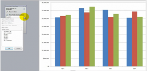
Interactive Pivot Table Chart

Interactive Pivot Table Chart

Pivot Charts in Excel 2007

In this lesson, I show you how to create a Pivot Chart in Excel 2007. Starting with Excel 2007, there are several major changes:

  • By default, Pivot Charts are embedded on the same worksheet as the Pivot Table Report that is linked to the chart.
  • A new, PivotTable Chart Filter Dialog box is available – this works “in tandem” with the filters available in the PivotTable Field List” Dialog box.
  • It is very easy to “Move” a Pivot Chart to its own worksheet tab – or vice versa – to move the Pivot Chart to an existing worksheet.

 Pivot Charts and Pivot Table Reports are Connected

A Pivot Chart MUST be connected to a Pivot Table Report. Any changes that you make to the chart are reflected in the report and vice versa. If you filter the Pivot Table Report, the filter is automatically applied to the Pivot Chart. This is an important concept to understand. This is the reason why it is so easy to make BOTH Pivot Table Reports and Pivot Charts “interactive!”

Explore My Index of Free Excel Video Lessons

I was surprised to discover that I had not yet created a video tutorial for Excel Pivot Charts when I looked at my list of “free” Excel Video Lessons. This became the impetus for creating this lesson. I invite you to explore all of my free Excel Video Tutorials. Click on this link to go to my Index of Excel Video Lessons. I have organized the free video lessons by topic. Simply click on the title of any lesson and you will arrive at the posting and the video for that lesson.

Download Excel File for This Lesson

View this Lesson in High Definition

I invite you to view this Excel Video Tutorial in High Definition, Full-screen Mode on my YouTube Channel – DannyRocksExcel

Watch Video Now


Feedback Welcome

I always welcome your feedback. Let me know what you think about this – or any other – video lesson. Add your comments below!

Extended Length Video Training Resource for Pivot Tables

I have created 90-minutes video training resources for Pivot Tables. Follow this link to learn more about my “Master Excel in Minutes” series.

Share and Enjoy:
  • Add to favorites
  • Facebook
  • Twitter
  • Technorati
  • Print
  • email
  • Digg
  • StumbleUpon
  • del.icio.us
  • Yahoo! Buzz
  • Google Bookmarks
  • Orkut
  • SphereIt
  • Sphinn

How to Convert a Pivot Table to a Standard List

Watch this video tutorial in High Definition on YouTube

A viewer aksed for my help. She has a boss and a few customers who:

  1. Do not know how to create or use Pivot Tables
  2. Have no desire to learn how to create and use Pivot Tables
Convert Pivot Table to Standard List

Convert Pivot Table to List

Nevertheless, in this example, she is being asked to create a summary report – by Year and by Quarter – from @ 5,000 daily transaction records. The fastest way to create this report is with a Pivot Table. Now, to meet the demands of her boss and clients, she needs to convert this Pivot Table into a standard list that can be Filtered and Subtotaled.

Summarize by Year and Quarter

To create this Pivot Table report:

  • Add the “Date” field to the grid and then select a single date.
  • Group the Date field by Month, Quarter and Year.
  • Add and arrange the Customer and Invoice fields to the Pivot Table Grid.

Convert Pivot Table to Standard List

  1. Remove both the Subtotals and Grand Totals from the Pivot Table Report.
  2. In Excel 2007 & 2010, ensure that you are using either the Outline or Tabular report layouts – NOT the new “default” Compact layout.
  3. Also in Excel 2007 & 2010, remove the Field Headers and the + / – Symbols.
  4. Now, select the entire Pivot talbe (use Ctrl + A) and copy it to the clipboard.
  5. Use Paste Special Values to paste the Pivot Table Results.

Filling the Blank Cells in the List

As you can see, whenever you have “nested rows” in a Pivot Table you get a nice, clean report. However, in order to Filter and Subtotal this new list, you will need to “fill in the blank cells.”

  1. Select all of the values and all of the blanks in Column A.
  2. Use Ctrl + G (or F5) to open the Go To Dialog Box and choose Special.
  3. From the Go To Special choices choose “Blanks.”
  4. With all of the Blank Cells selected use this formula: = ↑
  5. Do NOT press Enter. Rather, press Ctrl + Enter and all of the Blank Cells are now filled in with the Customer Names!
  6. Finally use Copy, Paste Special, Values to complete this process.

Watch This Video on My YouTube Channel – DannyRocksExcels

Since this video tutorial is a little longer than usual, I have decided to post it as a video – in High Definition – on my YouTube Channel. Click here to view it or copy and paste this link into your browser:

Link to YouTube Video:   http://youtu.be/IwReVDJ7BAI?hd=1

Download This Excel Workbook

Share and Enjoy:
  • Add to favorites
  • Facebook
  • Twitter
  • Technorati
  • Print
  • email
  • Digg
  • StumbleUpon
  • del.icio.us
  • Yahoo! Buzz
  • Google Bookmarks
  • Orkut
  • SphereIt
  • Sphinn

How to Create Custom Headers and Footers for Printing Excel Worksheets

How many times have you wasted time and paper when printing out an Excel Worksheet? Did you:

  • Forget to include the page numbers in the footer of each printed page?
  • Forget to repeat the column titles for the second and succeeding pages?
  • End up with “orphaned” columns that are disconnected from the main worksheet?
Headers and Footers in Excel

Headers and Footers in Excel

And the list goes on and on and …

Most Excel users, in my experience, spend very little time “previewing” their Excel worksheet prior to printing it – and wasting time and money. And also leaving a poor professional image in the minds of their clients and colleagues. 

Don’t let this happen to you!

Page Layout View

Page Layout View is a “working” view that was introduced in Excel 2007. I spend most of this video tutorial showing you how to get the most out of Page Layout View, including the placeholders for Header and Footer Elements. Personally, I spend a considerable amount of time when I am creating a new worksheet working in Page Layout View. Here, unlike in earlier versions of Excel, you can see how adding an additional column or two will effect the printed page. You can also verify that you company logo and other elements are properly positioned – while you are working inside the worksheet! For me, this view is indispensable!

Watch Video in High Definition on YouTube

This Excel Video Tutorial is a little longer than usual – 10 minutes and 14 seconds – and it contains more graphic images than usual. So, rather than embed this as an MP4 Video, I have decided to provide the link to this video on my YouTube Channel – DannyRocksExcels. Here is the link:

 http://youtu.be/X_Pb0KNFYak?hd=1

I produced this in High Definition, Full Screen Video Mode. This video is best watched on YouTube in High Definition. Let me know what you think.

Master Excel in Minutes – Not Months!

Learn how you can quickly learn how to get the most out of Excel – in the least amount of time! Click here to find out how!

Share and Enjoy:
  • Add to favorites
  • Facebook
  • Twitter
  • Technorati
  • Print
  • email
  • Digg
  • StumbleUpon
  • del.icio.us
  • Yahoo! Buzz
  • Google Bookmarks
  • Orkut
  • SphereIt
  • Sphinn

How to Apply Criteria for Advanced Filters in Excel

You want to use Excel to do more than just store data. You want to use Excel Filters in order to get information from your data set. In order to Filter the data, you need to create and apply criteria.

Options for Filtering Data:

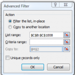
Advanced Filter Dialog Box

Advanced Filtering

  • Use the built-in AutoFilters – And, starting with Excel 2007 these include “Natural Language Filters!”
  • Use the Advanced Filter Dialog Box and your own Criteria Range – that is what I demonstrate in this lesson.

Now – since Excel 2007 – that the built-in filters include Date Filters, Text Filters and Number Filters, I do not use the Advanced Filter as much as in the past. However, there are at least two “must have” reasons to use Advanced Filters:

  1. To use “Calculated Field” criteria for your filters – e.g. to create a filter from a field that is not in your data set.
  2. To extract “Unique Records” that meet your criteria – and to copy them to another location.

I demonstrate both of these “must haves” in this video lesson.

How to Create an Advanced Filter

  1. Begin by inserting several blank rows above your Excel Data Set. These new rows will be used for your Criteria Range.
  2. Copy the Data Labels to the top row of your new Criteria Range. I like to link these with a formula – e.g. =A8 to maintain consistency with the Data Labels.
  3. Type or copy the values, comparison operators or formulas for your criteria in the row(s) below your criteria labels.
  4. Go to the Data Tab on the Ribbon and choose the Advanced Filter Command and use the Dialog Box Options.

Distinguish “OR” criteria from “AND” criteria

  • “OR” criteria use separate rows in your criteria range. You are selecting the records that match one OR more criteria.
  • “AND” criteria are written on the SAME ROW. You are filtering for records that match ALL the criteria on that row of your criteria range.

Computed Criteria in Filters

With Advanced Filters, you can use Computed Criteria for your filters. The formula must return a value that is either TRUE or FALSE. And the Label for your computed criteria CANNOT be the same as the labels in your data set.

In this lesson I show you how to filter for Invoices that have been paid – but paid “late” – after the “due date.”

Extract Unique Records with Advanced Filter

I show you how to copy the unique records – your list of customers – to a new worksheet. This is a great tip that I picked up by reading John Walkenbach’s books! Watch the video to see how this is done.

Watch My Video in High Definition

Click here to watch this video lesson in High Definition, Full Screen Mode on the DannyRocksExcels YouTube Channel.

Master Excel in Minutes Resources

I have created extended length video tutorials for Excel. I invite you to visit my online shopping website to: Learn how to “Master Excel in Minutes – Not Months!”

Share and Enjoy:
  • Add to favorites
  • Facebook
  • Twitter
  • Technorati
  • Print
  • email
  • Digg
  • StumbleUpon
  • del.icio.us
  • Yahoo! Buzz
  • Google Bookmarks
  • Orkut
  • SphereIt
  • Sphinn

Using the Built-in Excel Data Form to Edit, Enter and View Records

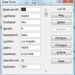
Data Form in Excel

Data Form

Excel has a built-in Data Form which is very useful for viewing all of the fields (up to 32 of them) associated with a single record. When you have lots of “Fields” in your “Data Set” and you do not want to do a lot of horizontal scrolling to view or edit the values in the cells, use this Data Form.

There is a limit of 32 fields when using Excel’s built-in Data Form.

Customize the Quick Access Toolbar

However, it does not appear as a Ribbon Command in Excel 2007. To use the Data Form add the Form Command to your Quick Access Toolbar (QAT) – I show you how to do this in the video.

Personally, I do not recommend the Excel Data Form for entering new records in your data set. I like to add Data Validation drop-down lists to ensure data integrity and this feature is not available in the Data Form. However, you can use Criteria to quickly find records for viewing and editing in the form.

Filtering Data with the Data Form

I give you a brief introduction to some of the new filtering options available in Excel 2007. I will cover this in greater detail in another lesson.

Subscribe to My Video Podcast on iTunes

I invite you to subscribe to my free video podcast, “Danny Rocks Tips and Timesavers” on iTunes. Click here to go directly to my iTunes podcast. I have had over 25,000 downloads since I began my podcast in June of 2010.

Watch this video in High Definition

Click here to go to my DannyRocksExcels YouTube Channel.

Watch Video Now

Master Excel in Minutes Video Training Resources

I have created a series of extended length Excel Video Training Resources. I invite you to visit my secure online shopping site to: Learn how to “Master Excel in Minutes – Not Months!”

Share and Enjoy:
  • Add to favorites
  • Facebook
  • Twitter
  • Technorati
  • Print
  • email
  • Digg
  • StumbleUpon
  • del.icio.us
  • Yahoo! Buzz
  • Google Bookmarks
  • Orkut
  • SphereIt
  • Sphinn

How to Use the SUMPRODUCT Function in Excel

In my experience, most Excel users are unfamiliar with the SUMPRODUCT Function. So let me give you two reasons to watch this short (5 minutes, 22 seconds) video lesson to learn how – any why – to use SUMPRODUCT:

  1. The SUMPRODUCT Function will speed up your calculations in Excel – get results with one step. With SUMPRODUCT() you can avoid several intermediary calculations.
  2. With SUMPRODUCT, you may be able to trim the size of your Excel worksheet. You may not need as many columns (fields) as you think to get the result that you need!

In this lesson, I show you how to calculate the Total Value of the Inventory (for a fictional company) with one formula!

50 Best Tips for Excel 2007

Excel Tips

Key Points Coverered

While the SUM Function “Adds Up” the values in the Arguments, the PRODUCT Function “Multiplies” the values in its Arguments.

  • Using “Arrays” in SUMPRODUCTS. In Excel 2007, you can use up to 255 Arrays! The key point is that all Arrays must be the same size and shape. For example, if the 1st arry in the Arguments is 15 rows in one vertical column, then all of the subsequent Arrays must be 15 rows in one vertical column.
  • I find that Creating – and Using – Names Cell Ranges for the Arrays will speed up writing the SUMPRODUCT formula.

I have decided to present the SUMPRODUCT Function in two lessons – so click on the sequel to see other uses for this function!

Click here to watch the 2nd video lesson on how to use the SUMPRODUCT Function in Excel.

You can watch this Excel Training Video Lesson in High Definition, Full Screen Mode on my YouTube Channel – DannyRocksExcels

You can learn how to “Master Excel in Minutes – Not Months!”

Share and Enjoy:
  • Add to favorites
  • Facebook
  • Twitter
  • Technorati
  • Print
  • email
  • Digg
  • StumbleUpon
  • del.icio.us
  • Yahoo! Buzz
  • Google Bookmarks
  • Orkut
  • SphereIt
  • Sphinn

How to Speed Up Data Entry on Forms By Using Named Cell Ranges

You can speed up data entry on an Excel form by creating – and using – named cell ranges. This also improves data accuracy, because the data entry clerk only has to hit the “Enter” key after each imput; the curosor automatically moves to the next cell in the named range that you applied to your form!

There is one “got’cha” step in this process. As you will see in this video, it is important to observe the position of the “Active Cell” in your selection!

The 50 Best Tips

The 50 Best Tips Series

Key Points Covered

  • Hold down the “Ctrl” key as you click on the cells in your non-contiguous range.
  • Use labels and cell shading to identify the cells that require data input.
  • When selecting your non-contiguous cells, choose the cell that you want to be the “Active Cell” last.
  • You can enter a formula or value into all of the cells in a range with “Ctrl+Enter.”

Try this out  on a form that you use at work. Remember to create a “name” for your data input cells. “Named cell ranges” are saved when you create a copy of your workbook – so this technique can be easily duplicated by saving the file with a new name.

Click here to watch this video in High Definition, Full Screen Mode on my YouTube Channel – DannyRocksExcels

Learn how to “Master Excel in Minutes – Not Months!”

Share and Enjoy:
  • Add to favorites
  • Facebook
  • Twitter
  • Technorati
  • Print
  • email
  • Digg
  • StumbleUpon
  • del.icio.us
  • Yahoo! Buzz
  • Google Bookmarks
  • Orkut
  • SphereIt
  • Sphinn

How to Name a Large Range of Non-Contiguous Cells in Excel

A client asked for my help on this problem. How to create a Named Range in Excel for Non-Contiguous Cells. The problem is that Excel puts a 255 character limit on the “Refers to” portion of a Named Range. I struggled with this until I found the answer in one of my favorite resource books, “This isn’t s Excel, it’s Magic!” written by Microsoft MVP (Most Valued Professional) Bob Umlas.

Solve the Problem

  1. Select the non-contiguous cells that you want to name.
  2. Open up the Visual Basic Environment (Alt + F11 is a Keyboard Shortcut).
  3. In the VBE, open up the “Immediate Pane” – Ctrl + G is the Keyboard Shortcut.
  4. Finally, type Selection.Name = “MyLabels” in the Immediate Pane and press Enter. (Substitute the name you want for “MyLabels”).

When you return to Excel, you will see that you can use the Drop-down list in the Name Box or in the Excel 2007 Name Manager to select this range.

 Amazing! Thanks Bob!

Additional  tips

  • Keyboard Shortcut F5 to open up the “Go To” Dialog Box. Select “Special” and choose “Constants – Text” to select the non-contiguous Labels that you want to name.
  • Right-click the worksheet tab and select “View Code” top open up the VBE (Visual Basic Environment) window.

I invite you to watch and subscribe to my Video Podcast on iTunes – follow this link to “Danny Rocks Tips and Timesavers”

Click here to watch this video in High Definition, Full Screen Mode on my YouTube Channel – Danny Rocks Excels

Learn How to “Master Excel in Minutes – Not Months!”

Share and Enjoy:
  • Add to favorites
  • Facebook
  • Twitter
  • Technorati
  • Print
  • email
  • Digg
  • StumbleUpon
  • del.icio.us
  • Yahoo! Buzz
  • Google Bookmarks
  • Orkut
  • SphereIt
  • Sphinn

Watch My Excel Videos in High Definition Full Screen Mode on YouTube

Logo for YouTube

YouTube Logo

At the request of several viewers, I have begun to produce my Excel, PowerPoint, Word, Outlook and Access Video Lessons in High Definition, Full Screen Viewing Mode. You can watch them, download them, share them and comment on them on YouTube. My YouTube Channel is DannyRocksExcels.

Here is the link to the YouTube”Playlist” that I have created for the HD Videos:

http://www.youtube.com/view_play_list?p=9D34C8C834E21A51

Please “bookmark” this link. As I add more HD Videos on YouTube, the Playlist will be updated.

My iTunes Podcast

Danny on iTunes

I will continue to post my videos on www.thecompanyrocks.com in M4V video format so that they can be sent automatically to the iTunes store. I invite you to subscribe to my video podcast – Danny Rocks Tips and Timesavers – on iTunes. It is free! Here is the link to my iTunes podcast:

http://itunes.apple.com/podcast/danny-rocks-excel-tips/id374923275

I welcome your feedback on my videos. Let me know what you like, what you don’t like or would like to see improved. Send me your questions and I will do my best to answer them promptly. Just drop a note to say hello!

Learn how to “Master Excel in Minutes – Not Months!”

Share and Enjoy:
  • Add to favorites
  • Facebook
  • Twitter
  • Technorati
  • Print
  • email
  • Digg
  • StumbleUpon
  • del.icio.us
  • Yahoo! Buzz
  • Google Bookmarks
  • Orkut
  • SphereIt
  • Sphinn

How to Add a Check Box Control to an Excel Form

Judging by the comments that I get from many clients, adding a “Check Box Control” to and Excel Form is not as easy as it appears at first glance.

And, I agree! I, too, struggled with adding Form Controls in Excel. Most of the explanations that I read seemed to add more confusion than clarification!

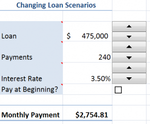
Spin Buttons in Excel

Spin Button Controls

That is why I created this Excel Training Video: to  lead you through the process; to save you some time and to ease your frustration.

Key Points to Remember:

  1. In Excel 2007, be sure to display the “Developer Tab” on the Ribbon in order to to Insert any Form Control.
  2. Choose the Controls in the “Forms Controls” and NOT in the Active X Controls.
  3. After you “draw” the Control Box on your Form, be sure to select a “Cell Link” to enable the Check Box Control.
  4. Remember that a Check Box Control can only be applied when the result of the Formula or Option is a Logical Value – either a result of  “True or False.”

Don’t be scared off! I find that this is an Excel concept that is better presented “visually.” I struggled for some time when I “read” how to add form controls.

So … I welcome your thoughts – “True or False.” Did I make this easy for you to understand?

Please feel free to add your comments below!

Watch My Video on YouTube

Follow this link to watch my tutorial on my YouTube Channel – DannyRocksExcels

Watch Video Now


Master Excel in Minutes Training Resources

I have created a series of extended length Excel Training Videos. I invite you to visit my secure online shopping site to:

Learn how to “Master Excel in Minutes – Not Months!”

Share and Enjoy:
  • Add to favorites
  • Facebook
  • Twitter
  • Technorati
  • Print
  • email
  • Digg
  • StumbleUpon
  • del.icio.us
  • Yahoo! Buzz
  • Google Bookmarks
  • Orkut
  • SphereIt
  • Sphinn