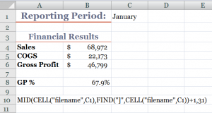
Dynamically Update a Cell with an Excel Worksheet Name

Capture Tab Name in Cell

I am excited to share this Excel Tip with you! Several viewers have recently asked if there was a way to create a link in a cell to the name of a worksheet tab. Yes there is! And, in this lesson, I demonstrate how to do this.

Say, for example, that you want Cell C1 to contain the name of the current worksheet (Sheet1). With this formula, when you change the name of the worksheet to “January,” cell C1 is dynamically updated to show “January.”

Perfect for Excel Templates

If you use a template for your monthly, regional sales or financial reports, then this Excel formula is essential. You write the formula once – using Group edit – and each worksheet in your Excel workbook will be linked to a cell in your report. Change the name of the worksheet and your report name is automatically updated.

Functions Used in this Formula

CELL() – to gather information about the worksheet – in this case, the “Filename.”
MID() – to extract the characters in a text string – e,g, the “worksheet name.”
FIND() – to locate the starting point for the MID() function to extract the characters in the text.

As the final argument for the MID() Function, I use 31 characters because that is the maximum number of characters that you can use when naming an Excel worksheet.

Try this for yourself. Let me know how it works for you. Add your comments below.