Be Careful with Calculated Items in Pivot Tables

Let me warn you – Calculated Items in Pivot Tables can produce incorrect results! Calculated Items can be useful – in special circumstances. However, don’t use a Calculated Item to create a Quarterly Summary. It is too easy to accidentally “double” your sales! And, this will not earn you any special bonus. In fact, it may harm your reputation as an Excel expert. So be very careful before you create a Calculated Item.

Review my Excel Training Video on Grouping Data to see the preferred way to produce a Quarterly Summary in a Pivot Table.

Here are the steps to follow in this lesson:

  1. You use a Formula to Calculate an Item from the values on one of the Fields in your Pivot Table.
  2. Select one value in the Field where you want to create the Calculated Field.
  3. In this lesson, I selected a Month and then from the Drop-Down Menu on the Toolbar I chose Formula – Calculated Item,
  4. I named the Calculated Item Q1 (1st Quarter) and for the Formula I clicked = January+February+March. Click Add and then click OK.
  5. As you can see, the new Q1 Item actually “doubled” the existing sales for January – March. That is not what you were looking for!
  6. To remove the Calculated Item, select it and then from the drop-down select Formulas – Calculated Item. Highlight Q1 and click Delete – OK.
  7. Review my video to see how to Group Data to produce the Quarterly Summary in the Pivot Table.

Search My Index of Excel Training Videos to find the topic you want to view

DVDs of The 50 Best Tips for Excel and PowerPointNew! Danny’s DVD Training Series, “The 50 Best Tips for …” is now available at the online store for The Company Rocks

Group Data in Pivot Table for Quarterly Report

During a recent Excel training class, one student asked me if was possible to create a Quarterly Summary Report in a Pivot Table. Yes, it is quite easy to do this – as you will see in the video.

In the Data Set that we are using for this Pivot Table we have four territories and 12 months of sales for each territory over a one year period. The Months (Jan, Feb, etc.) are not actual dates (e.g.1/1/08,) they are Labels.

In an earlier video, I showed you how easy it is to create new fields for Months, Quarters & Years from a Date field. Because our months are Labels, we will GROUP the Months to create the 1st, 2nd, 3rd, and 4th Quarters in our Pivot Table.

Here are the steps to follow in this lesson:

  1. Create a Pivot Table using the default settings in the Pivot Table Wizard. Place the Months in the Row area, the territory in the Column area, and the Sales in the Data area.
  2. Select the Labels January, February, March. On the Pivot Table drop-down menu select Group & Show Detail – Group.
  3. Rename the generic label (Group1) to 1st Qtr.
  4. Follow the same sequence of steps to create Groups for the 2nd, 3rd, and 4th Quarters.
  5. Rename the new, generic field (Month2) Quarter.
  6. Use the Toolbar Commands to Hide & Show Detail as desired.

NEW! Download the Excel Practice file that I used in this video

Search the Index of Excel Lessons to find my training video listed by topic

New! Danny’s DVD Training Series, “The 50 Best Tips …” is now available at the online store for The Company Rocks

Related Videos

I Added a New PowerPoint Video Lesson

I am just getting back to adding more PowerPoint Video Lessons on my blog. Follow this link to view the video – “Tools To Control Text On Slides”

The key learning points in the lesson:

  • Enforce a style to limit the number of bullet points per slide.
  • Establish a style to maintain consistent ending punctuation (on or off) for bullet points.
  • Establish minimum font sizes for Slide Titles and bullet points.

Reduce “Visual Clutter” on your PowerPoint slides. Achieve the professional look that sets you apart from other presenters. Use the tools that PowerPoint provides to help improve Visual Clarity.

Tools To Control Text On Slides

I want you to reduce the “Visual Clutter” on your PowerPoint Slides. You are not trying to write a “ransom note,” you are attempting to create a professional image.

PowerPoint has a great set of tools that you can use to enforce the Visual Style options that you set. In this video lesson, I demonstrate how to set up the style guides and then how to use PowerPoint’s tools to make the changes that conform to your rules.

Here are the steps to follow for this lesson:

  1. Go to the Tools Men and choose Options and then click the Spelling & Style Tab.
  2. On the Spelling & Style Tab choose Style Options.
  3. You can make your stylistic choices on the “Case & End Punctuation” tab and on the “Visual Clarity” tab. When you have made your choices, click OK.
  4. Back in Normal View, when you click in a Text Place holder, look for the Yellow Light Bulb. Click on it to see your options to conform to the style settings that you set.
  5. Also, look for the AutoFit Options Smart Tag. Choose the best option to change your style.

Search my Index of PowerPoint Video Lessons for the topic of your choice.

News! My DVD, “The 50 Best Tips for PowerPoint 2007” is availabe for purchase. Visit my online store for details.

Related Videos

Three Frustrations When Calculating TIme in Excel

When I am training a class to use MS Excel, I always get at least one question about performing time calculations. I sense that the person asking the question is frustrated. When I ask, “How many of you are frustrated when you try to perform a calculation to total time periods in Excel?” nearly every hand is raised! And they are right; Excel’s time calculations can cause frustration.

In this video lesson, I will show you how to overcome three common frustrations that you may have when performing time calculations in Excel.

Here are the steps to follow in this Excel Training Video:

  1. Format the cell that contains the formula =End_Time – Start_Time) to the Custom Number Format h:mm
  2. I encourage you to use this formula instead of a simple formula: =IF(End_Time < Start_Time, End_Time + 1, End_Time)-Start_Time.
  3. This will eliminate any possible “Negative times” which result in a cell filled with ######### A Negative Time is frequently the result of “Time Periods that Span Midnight. e.g. Start @ 11:00 PM and End @ 3:00 AM
  4. TIP: Use this Formula =MOD(End_Time – Start_Time, 1) This is the MODULUS Function.
  5. When you calculate the total number of hours and the result exceeds 24 hours, use this Format [h]:mm

Search My Index of Excel Video Lessons

 “The 50 Best Tips for …” is now available at the online store for The Company Rocks

Related Videos

How to Create Scenarios in Excel

Scenarios are part of Excel’s “What-If” Analysis tool set – aka Data Analysis. Use Scenarios when you need to know what the result will be when you change one or more variables in one or more  situations (scenarios).

Frequently, I create Scenarios to define  a “Good, Better, Best” or “Worst Case, Best Case, Case Most Likely” outcome.

In this short Excel Training Video, I demonstrate how to create, edit,  and report four Scenarios for a Monthly Office Expense Budget.

These are the steps used in this Excel Video Lesson:

  • Create (or open) an Excel worksheet that contains a formula. Identify the formula and the precedent  cells that feed into the formula.
  • Select the “target cell” – the cell that contains the formula whose result will change with each Scenario.
  • Choose TOOLS – SCENARIOS and follow the directions in the Create Scenario dialog box.
  • First, click ADD. Name the Scenario. Click OK. Confirm that you have selected the “Target Cell” and then click / type in the “Changing cells.” The Changing cells should be either direct or indirect precedents to the Target cell formula. Click Add. Add additional Scenarios as desired.
  • Click on the name of your Scenario and select SHOW to display the changing cell values and the new result in your target cell.
  • If you wish, choose SUMMARY to create a summary report in a separate worksheet.
  • I strongly recommend that you create named cells and use them in the formulas and changing cells of your Scenario.

NEW! Download the Excel Practice file used in this lesson:

Use my Index to search for the free Excel Training Video that you want to view.

New! Danny’s DVD Training Series, “The 50 Best Tips …” is now available at the online store for The Company Rocks

Related Videos

12 Excel Practice Files to Download

I want to thank the viewers who emailed me and responded to the Poll on this blog. I have now uploaded 12 Excel Practice files to this blog. Follow this link to navigate to the Download Excel Practice files page.

  • Click on the Practice file that you are interested in.
  • Right-click the Icon to determine how and where to open the practice file.
  • The Practice files are saved as “Interactive Web Pages.” From here, you can decide to work with the file over the Internet or to save it to disk as an Excel Workbook.

I will be adding additional Practice files – approximately three each week – so check back to locate the latest files that I have downloaded. If there is a particular file that you want to work with, email me your request – danny@thecompanyrocks.com and I will make it available as quickly as I can.

Thank you for your continuing support of The Company Rocks!

Sorry, there are no polls available at the moment.

My Favorite Excel Keyboard Shortcut

I use Keyboard Shortcuts in Excel everyday. However, the one that I count on the most; The one that has saved me from near disaster on multiple occasions is:

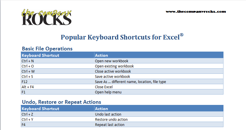
Ctrl + Z – The UNDO Command.

Ctrl + Z can Undo my last 16 actions (one at-a-time.) In Excel 2007, you can Undo up to 100 of your last actions!

Watch this short Excel Training Video as I demonstrate how to take advantage of the Ctrl + Z Shortcut.

Here are the steps to follow in this lesson:

  1. Type an entry or apply formatting to a cell or range of cells.
  2. Hold down the “Ctrl” Key while you press the “Z” key. Excel will Undo your last action.
  3. To Restore the Action that you just UNDID, use the “Ctrl + Y+ Keyboard Shortcut.
  4. You can Undo your last 16 actions in Excel 2003. Use the drop-down menu next to the UNDO Command Button on the Standard Toolbar.
  5. Follow a similar  procedure to RESTORE up to your last 16 actions in Excel 2003 with the drop-down menu next to the Restore Command button on the Standard Toolbar.
  6. In Excel 2007, you can UNDO and RESTORE up to your last 100 Actions!

Are you looking for Excel Video Training for a specific topic? Search my Index of Excel Video Topics.

Related Videos:

NEW! Now you can practice your Excel Skills – Download the Excel Workbooks that I use in my video lessons

How to Publish an Excel Workbook as a Webpage

How good is your information – if you or your colleagues can not access it when you need it?

Not good enough!

I love USB Flash Drives for their portability. But, when I need – or I need to send an Excel Workbook – halfway around the world …? I need a better way to access that information.

I need to learn how to publish my Excel workbook as Web page – complete with Interactivity. Watch this short video lesson as I demonstrate how to:

  1. Save an Excel Workbook as a Web-page – be sure to enable Interactivity.
  2. Add, edit and delete data in the workbook while on-line.
  3. Send the Webpage version of the workbook back to Excel – to communicate my changes or to further analyze the data.

News! My DVD, “The 50 Best Tips for Excel 2007” is now availabe to purchase. I invite you to visit my online bookstore for more details.

Related videos

Looking for the solution to an Excel problem? Search my Index of Excel Video Lessons.

What is an Interactive Excel Workbook? Please Vote

I created this short video for two reasons:

1)  To demonstrate what an “Interactive Excel Workbook” looks like. Interactive Excel files are “published” to an Internet or Intranet browser. You save an Excel Workbook as a “Web Page.” Adding “interactivity” is an option that you can select.

Notice that there are no Menus and there is only one toolbar. Also, you activate the other worksheets in a different way.

I am happy to make these Practice files available to you – if there is sufficient interest.

2) Please signify your level of interest by taking the POLL on the sidebar of this page. It is fast and easy – there is only one question; and only one choice, “Yes” or “No.”

I hope to hear from you!

Go to my new page to download the Interactive Excel Practice Files
Thanks in advance!

Danny Rocks

News! My DVD, “The 50 Best Tips for Excel 2007” is now available to purchase. I invite you to visit my online bookstore for more details.