Select Excel Data with Keyboard & Mouse-click Shortcuts

During a recent training class, I demonstrated several Keyboard and Mouse-click shortcuts for selecting and finding data. Several people in the class had “A-Ha” moments. So, I created this video lesson to share these shortcuts with you.

Here are the steps to follow in this Excel Video Lesson:

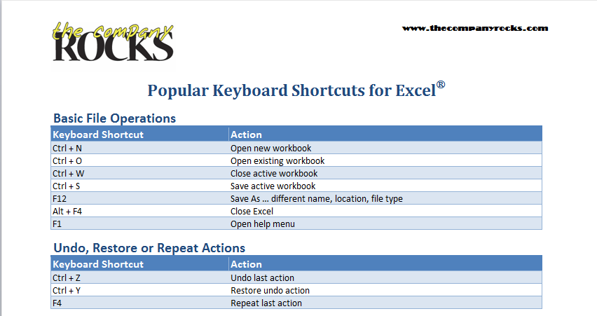
  1. To select all of the contiguous data cells, make one cell the “Active Cell”. Ctrl+A will then select all of the cells in that data block.
  2. If you then click Ctrl+A a second time, you will select every cell in the worksheet. This is handy when you need to “AutoFit the column width in the worksheet.
  3. Use Ctrl+End to go to the last cell in your data set. Ctrl+Home will return you to the Top cell in the data set.
  4. To find a blank cell in a column, position your mouse at the bottom of the “active cell” and double-click. This takes you to the last cell that contains data in that column.
  5. To select all of the cells w/ data in a column use the Ctrl+Shift+ Down Arrow. Use the appropriate Arrow Key to select cell containing data in a Row.
  6. Quickly copy a Formula to all of the cells in the column. Position the mouse in the lower right corner of the cell with the formula and double-click.

News! My DVD, “The 50 Best Tips for Excel 2007” is now available to purchase. I invite you to visit my online bookstore for more details.

Related Videos

Find a specific Excel Video Lesson – Index of Excel Video Lesson Topics

NEW! Download the Excel Workbook file that I used in this lesson:

Related Video Lessons

Change Pivot Table Grouping to a Fiscal Quarter

While I was training a class to use Pivot Tables this week, I showed them how to Group Dates by Month, Year & Quarter. They liked that a lot – it’s a great feature! However, one student said, “My company is on a Fiscal Year. Is it possible to change the grouping of the Quarters from a Calendar Year to a Fiscal Year?”

Yes! There are several ways to do so. In this Excel Video Lesson I demonstrate the easiest way.

Here are the steps to follow in this Excel Training Video:

  1. Create the Pivot Table. In this example we drag the “Date Field” to the “Row Area” and drop the “Sales Field” into the “Data Area.”
  2. Select one cell in the Date field and from the Pivot Table drop=down menu choose Group & Show Detail – Group. Highlight Month & Quarter. Click OK.
  3. We now have a new “Outer Row” filed – Quarter – in our Pivot Table. However, the grouping reflects a Calendar Year. We need to change this to a Fiscal Year.
  4. Select each label, in turn, and edit the name in the Formula Bar.
  5. To change the Order of the Quarters: Right-click the 4th Quarter label and choose Order – Move to End.
  6. Edit the Field Settings for the Quarters Field. Add in the SUM Subtotal.
  7. Make the Quarterly Subtotals & Grand Total rows Bold.
  8. Double-click any Quarterly Label to Hide the Details. Use the Icons on the Toolbar to Show / Hide details for each group to suit your needs.

Looking for a specific Excel Video Lesson? Click here for an Index of all Excel Training Topics

Do you want to see a list of all of my Excel Pivot Table Video Lessons? Click here to go to my Pivot Table Archive.

News! My DVD, “The 50 Best Tips for Excel 2007” is now available to purchase. I invite you to visit my online bookstore for more details.

Viewer Request: How do I calculate dates in the future?

Today’s lesson is my answer to a viewer’s question: “How does Excel calculate a date in the future?”

The viewer wrote me because they were having trouble writing a formula that would return a date “N-Months” in the future. Or “3 years in the future” from a specific starting date.

I am asked this question frequently. In this short Excel video lesson I demonstrate how you write the formula.

Here are the steps to follow in this Excel Training Video:

  1. Use the AutoFill feature and Options to increment your “Starting Date.” I recommend using your “right-mouse button” to AutoFill because it automatically brings up a Menu of Options when you release the Right-Mouse Button.
  2. In response to the viewer’s question, we will choose “Fill Months.”
  3. Remember that we are using a “Hard-Coded” date as our “Starting Date,” so each value is really a “constant value.” This may not be the optimal result that we are seeking.
  4. In order to provide flexibility (with your starting date) you need to learn how to construct a formula that will increment (in this case the MONTH) our values.
  5. Use the “DATE() Function.
  6. For each of the “Arguments,” use the YEAR(), MONTH() and DAY() functions.
  7. To answer my viewer’s question we use MONTH(A2) +1 in the “Month Argument.”
  8. To “Increment the Year,” we use YEAR(A2) +1 in the “Year Argument.”
  9. Finally, write a “Formula” to verify that Excel is properly accounting for “Leap Years.”

Search My Index to all Excel Video Training Topics

The 50 Best Tips for Excel 2007″ DVD is now available for purchase. I invite you to visit my online bookstore for more details.

Consolidate Data as a Quick Alternative to Subtotals

I have a great tip for you! When you need to produce a quick summary report of your data, use Consolidate in place of Subtotals. Here’s why:

  • You don’t have to sort the data when you consolidate.
  • You can use multiple functions (SUM, AVERAGE) in adjacent columns in your report.
  • You can easily copy and paste the Consolidated Summary Report to another workbook or into Word.

Watch this short video as I demonstrate how to use Data Consolidate in place of Subtotals.

Steps to follow in this lesson:

  1. Select an empty cell. Choose Data – Consolidate.
  2. In the dialog box, choose the Function that you want (SUM is the most common) and then select your data range (including the Column Headers) and click ADD.
  3. Be sure to check the Use Labels in “Top Row” and “Left Column.” Click OK
  4. A quirk – The Label for the Category does not appear when you Consolidate Data – Simply copy & paste it from cell A1.
  5. Repeat these steps to add an additional Function – e.g. AVERAGE to your Consolidation Report.
  6. Copy and paste the Consolidated Data to another workbook or to another application – e.g. MS Word.
  7. Contrast this quick alternative to creating Subtotals.
  8. The real “Time Saver” comes from the ability to quickly copy the Consolidated Summary.
  9. The “Gotcha” to remember with Subtotals is to choose “Edit – Go To – Special – Visible Cells Only” before you copy the Level 2 Subtotals. If you omit this step, you will discover that you have copied ALL of the data and not just the summary!

Find the Excel Training Video that you want – Click here for the Index to all Excel Topics

Learn how to “Master Excel in Minutes – Not Months!”

Use the =SUMIF() Function to Tally YTD Sales

Many of my clients keep a “running total” of sales. They put “Dates” in Column “A” and enter each day’s sales in Column “B.” Next is Column “C” which contains the formula =SUM(B$:B250). That is fine – it works.

However, if you use the =SUMIF() function to total Year-to-Date (YTD) Sales you gain flexibility, save space and save time – because you do not have to scroll down several screens to see your YTD Sales total!

In this video, I show you how to use “Named Ranges” in a =SUMIF() Formula to keep track of your cumulative sales total.

Here are the steps to follow in this lesson:

  1. Traditionally, you use a formula like =SUM(B$3:B250) to give you a “running total” for YTD Sales.
  2. The=SUMIF() Function returns the SUM of vales that meet a “Single Criterion” (the IF portion) .
  3. The 1st Argument is – What is the Range that you want your criteria to evaluate? Consider “Naming” this Range – it makes it easier to write your formula and explain your formula.
  4. The 2nd Argument is – What is your criteria? Be sure to use this syntax – “Comparison Operator”
  5. In the video example we also need to include the “&” to join the cell “D2.” Cell “D2,” in this example, contains the Function =TODAY()
  6. The 3rd Argument is – What Range do you want to SUM to return the values that meet your Criteria?
  7. The =DATE() Function returns the serial number for a specific date. It requires 3 Arguments. =Date, Year, Month, Day)
  8. You will save time and gain productivity when you “Name Cells and Ranges” and then you them in your formulas.
  9. Use the F3 shortcut key to “Paste Names” into your formulas.

News! My DVD, “The 50 Best Tips for Excel 2007” is now available to purchase. I invite you to visit my online bookstore for more details.

Find the Excel Video Lesson that you want – Index to all Excel Topics

Click & Drag a Data Series to Goal Seek in Excel

Did you know that you can click on a Data Series in an Excel Chart and “drag it to reach a new value?” You can!

Changing the data value in your chart brings up the Goal Seek Dialog Box. Now, it is a simple matter to confirm your new value and tell Excel which cell reference to change in your formula. Instantly, your chart redraws and your data and formula are updated with the substitute value – and your NEW GOAL!

Here are the steps to follow in this Excel Video Lesson:

  1. I use the =FV() Function to show the future value of my investment for each year that we invest. The =FV() Function requires a “fixed” interest rate and a constant investment value contributed each period.
  2. I inserted a “Line” type chart onto my worksheet – i.e. I “embedded” the chart on the sheet.
  3. I used a “Custom Format” on the Value Axis for our numbers (#,##0,K) to show the numbers as thousands ($80K)
  4. For this chart, I also changed the “Maximum Value” of the Value Series by typing in a new (higher) number.
  5. To reach a “new goal” on our chart, first click to select the data series. Then click again and drag the data line to a new point on the chart.
  6. This brings up the “Goal Seek” Dialog Box. Edit your new goal if necessary. Then click on the cell that you want to change in order reach your goal. That cell must be referenced in your formula. The chart redraws and your formula results are updated.

Find the Excel Video Lesson that you want – Index of all Excel Topics

News! My DVD, “The 50 Best Tips for Excel 2007” is now available to purchase. I invite you to visit my online bookstore for more details.

Excel Tells You the Future Value of Your Investment

Hey, want to know what your investment will be worth in 5 years? 10 years? Want a sure thing? Excel correctly calculates the future value of any investment! Provided …

  • You make a series of regular investments – even if it is just one “lump sum.”
  • The interest rate that you earn is “constant” – that is a “fixed annual interest rate.”

OK, so now you understand that neither I nor Excel are “touting sure thing” winners in the stock market. No one can do that. But, you can’t beat Excel when it comes to accurate – and easy to use – financial calculations.

In this video lesson, I demonstrate how to use both the =FV() and =PMT() Functions to calculate Future Values. I also show you how to perform “What-If” Analysis using a One-Input Data Table.

Here are the steps to follow in this Excel Video Lesson:

  1. Input values for Interest Rate (RATE), Number of Periods (NPER) and your Investment (PMT). These are the three required arguments for the =FV() Function. Use the Function Argument Dialog Box to ensure that you use the correct syntax for this function.
  2. One of the “optional” arguments is “Type.” If you omit this, Excel defaults to a “0” which means that you will make your investment contribution at the end of each period. A “1” means that the contribution is made at the beginning of each period. Over a number of years, this can make a significant difference in the “Future Value” of your investment.
  3. FV is also an “argument” in the =PMT() Function. If you want to calculate how much you need to contribute each month to reach a Savings Goal, use the =PMT() Function. However, in this case, the FV – while showing as an “Optional Argument” will refer to the cell containing your Savings Goal.
  4. Create a One-Input Data Table to perform “What-if” Analysis – e.g. to substitute a series of different interest rates in your =PMT() – or =FV() Function.

NEW! Download the Practice File for this Excel Video Lesson:

Find the Excel Video Lesson you want – Index of all Excel Topics

News! My DVD, “The 50 Best Tips for Excel 2007” is now available to purchase. I invite you to visit my online bookstore for more details.

How to Create a Combination Chart in Excel

What is a Combination Chart? When do I use one? Why do I use one?

  1. What: A combination chart uses two different chart types in the same graphic representation of your data.
  2. When: There is a large value gap between one data series and the other data series.
  3. Why: To reveal the relationships in your data that may not be apparent with a traditional chart or by merely examining the data.

In this short video lesson, I will demonstrate “How” to transform a traditional column chart into a Combination Chart that reveals an interesting data relationship.

Here are the steps to follow in this Excel Video Lesson:

  1. Start with a standard Excel Chart – Here we used the F11 Key to create a Column Chart in a separate worksheet.
  2. Notice the wide gap between the two data series. Click on one of the series columns (in this case “Dollars”) and on the Chart Toolbar select the “Line” chart type.
  3. A wide gap in values remains between the two series. With the “Dollars” series selected, choose Format Series on the Toolbar. Click the Axis Tab and select “Plot Series on Secondary Axis.”
  4. Format the chart to suit your needs. In this example, we change the color of the Plot Area and add Text to a “Call out” shape on the chart.

Find the Excel Video Lesson that you want. Index of all Excel Topics

News! My DVD, “The 50 Best Tips for Excel 2007” is now available to purchase. I invite you to visit my online bookstore for more details.

Related Videos

How to Explode a Pie Slice in Your Chart!

Pie Charts are the most popular charts – to create. Pie Charts are not always the best chart to use to tell your story. The people who create charts want to create Pie Charts and they want to “Explode” slices of the pie.

In this video I will demonstrate how to format your Pie Chart – and “explode” it!

Here are the steps to follow in this Excel Video Lesson:

  1. Select the chart first so that you can format it. (If your chart is on its own worksheet, select that worksheet tab.)
  2. Use the Drop-Down menu on the Chart Toolbar to become familiar with each Chart Element.
  3. Select the Chart Element and then click the Format Chart Element Icon on the toolbar.
  4. Format the “Plot Area.” Remove the Border and change the Background to White.
  5. Select the Chart Series “Total” – the Pie – and format it. On the Data Labels tab, select Percentage and Category Names.
  6. You no longer need the Legend. Select it and press Delete.
  7. Select the Plot Area and drag the sizing handles to enlarge it.
  8. To “explode” a pie slice, first select the Series “Total” – the Pie. After a short pause, select the slice that you want to “explode” to choose it. (You will see multiple “handles” around this slice.) Click on the border of the slice and drag it away from the Pie.
  9. To print only the chart: Select it and then make your changes in Print Preview – Page Setup.

Find the Excel Video Lesson that you want – Index to all Excel Topics

News! My DVD, “The 50 Best Tips for Excel 2007” is now available to purchase. I invite you to visit my online bookstore for more details.

Related Videos

Create an Excel Chart With One Keystroke!

It is easy to create a chart in MS Excel 2003. So easy, in fact, that you can create your chart with one keystroke.

In this video, I reveal that keystroke. I also demonstrate how easy it is to change the chart type and the location of your chart.

Here are the steps to follow in this Excel Video Lesson:

  1. Select one cell in your data set and press the F11 key.
  2. Excel, by default, creates a Column Chart in a new worksheet.
  3. Using the Chart tool bar, you can change the chart type.
  4. Select the data range(s) you want to chart  before you press the F11 key.
  5. Consider what “picture” you want to share before you create your chart.
  6. Use the Chart Wizard – Step 4 – to move the location of the cart (from its own worksheet to an embedded object in your worksheet – or vice versa.)

Find the Excel Video Lesson that you want – Index to all Excel Topics

News! My DVD, “The 50 Best Tips for Excel 2007” is now availabe to purchase. I invite you to visit my online bookstore for more details.

Related Videos