How to Roll Up a Summary by Month to Filter an Excel Pivot Table

Filter Using a Roll Up by Month Summary

Filter with a Roll Up by Month Summary

In this Excel tutorial, I respond to a viewer request. He likes the new “Roll Up Summary by Month” feature for filtering a field in an Excel 2007 – 2010 Field. What he finds frustrating – there seems to be no natural way to accomplish this with an Excel Pivot Table.

Natural Language Date Filters in Excel

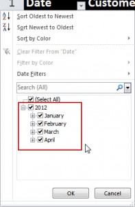
Before I solve my readers dilemma, I demonstrate how to take advantage of the new “Natural Language” Date Filters that were introduced in Excel 2007. Date Filters allow you to filter records from “Today,” “Last Week,” “Next Month,” etc. They are available for Excel Tables and Excel Pivot Tables. These “Natural Language” Date Filters are a major improvement in Excel!

Group a Field for Pivot Tables

To solve my viewers question, I “Grouped” the original Date Field in his Pivot Table to produce “virtual” fields for “Month,” and “Year.” Now, it is a simple step to filter the “virtual” Month Field to obtain a “roll up” filter for individual months in the Pivot Table. Just select a single cell in the Pivot Table Date Field and choose Group Field. Make your choices in the Grouping Dialog Box and you are “good to go!”

I also show you how to take advantage of the Expand and Collapse Field Commands in a Pivot Table.

In-Depth Video Tutorial for Excel Pivot Tables

At my secure, online shopping website, you can purchase my 90-minute Video tutorial for Excel Pivot Tables. Available for immediate downloading or on a DVD-ROM. Version specific editions for Excel 2003, 2007, and 2010.

Watch Video Tutorial in High Definition

Follow this link to watch this tutorial in High Definition Mode on my YouTube Channel – DannyRocksExcels


How to Analyze Point-of-Sale Data with an Excel Pivot Table

Advantages of Pivot Tables

Advantages of Pivot Tables

This is the first in a series of tutorials that I am creating in partnership with Tri-Technical Systems – a leading provider of Point-of-sale (POS) Systems. In this video lesson, I use an Excel Pivot Table to present the information that I require from a standard “Inventory by Location” report.

Point-of-Sale Reports

Most POS Systems allow you to print out standard reports – compact, professionally formatted “snapshots” of your inventory status, sales data and customer information. Likewise, most POS Systems will allow you to easily export the data behind these reports to Excel – where you can analyze or “number crunch” the data.

Advantages of Pivot Tables

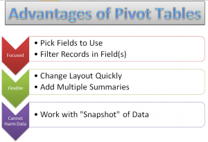
  • Pivot Tables combine the best elements of Subtotals, Outlines and Filtered Reports.
  • With a Pivot Table, you select only the Fields that you wish to focus on.
  • You can quickly reposition any field on your Pivot Table – e.g. change it from a Vertical to a Horizontal position.
  • Pivot Tables allow you to easily add multiple summaries – e.g. Sum, Average, Percentage of Total, etc. without writing a Formula!
  • It is impossible to harm your underlying data when you work with a Pivot Table because you are working with a “virtual snapshot” of your data. You cannot directly change any value in a Pivot Table Report!

Learn More About Pivot Tables

Pivot Tables are easy to learn. However, it does take practice if you want to really tap into the analytical power of  a Pivot Table Report. Fortunately, I have a great resource for you – a 90 minute focused video tutorial on Pivot Tables. Follow this link to go to the information page for my Excel 2010 Pivot Table DVD-ROM. I have also created Pivot Table videos for Excel 2007 and Excel 2003.

Watch Tutorial in High Definition

You can watch this Excel Tutorial in High Definition on my YouTube Channel – DannyRocksExcels

View My Video Now