Create a Pivot Chart to Present a Frequency Distribution Report

Combination Chart for Frequency Report

Quite a few of my viewers requested that I continue my series of creating and presenting a “Frequency Distribution Report” using an Excel Pivot Table. So, here is the new Part 3 in the series!

In this Excel Video Tutorial, I demonstrate – using Excel 2010 – how to create a Pivot Chart for the Frequency Distribution Pivot Table that I created and modified in Parts 1 and 2 of this series.

Key Point: A Pivot Chart Must be based on a Pivot Table Report!

  • Any structural changes that you make to the Pivot Table are reflected in the Pivot Chart.
  • If you “filter” the Pivot Chart, those filters apply to the Pivot Table that is the basis for your Pivot Chart – and vice versa.

Focus on the Chart

As I demonstrate in this video – posted on YouTube – I prefer to focus on one task at a time. I prefer to get the formatting and structure of the Chart “right” before I think about using Filers and other “goodies to add .” This “Best Practice” helps me to get more accomplished in less time!

My bottom line is: “Focus on the task at hand. Eliminate any possible distractions from that primary task!”

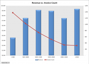
A correctly designed Pivot Chart will help you to present your information accurately and interactively! For this presentation, I decided that a “Combination Chart” would be the best way to present the information that I wanted to convey. A “Combination Chart” allows you to have a Primary Axis (Revenue) that uses a Column Chart Type and a Secondary Axis (Invoice Count) that uses a Line Chart Type.

When to Use a Secondary Chart Axis

In this example, there is a wide difference between the two fields that we are charting:

  • Revenue for the Invoices in the “Bin Range” is in “the millions!
  • Count of Invoices in the “Bin Range” falls into the hundreds and low thousands.

Using a “Combination Chart” in this example – (Column Chart for Revenue in Millions) and Count of Invoices (Line Chart for Count in Hundreds) allows you to present the “relationship” between both metrics. I show you step-by-step how to create this combination chart!


Watch This Video in High Definition on YouTube

Follow this link to view this video tutorial in High Definition on my YouTube Channel – DannyRocksExcels

Click this link to view Part 1 of the 3 Part series – Creating a Frequency Distribution  Report with Excel Pivot Table

Click this link to view Part 2 of the 3 Part series – Formatting a Frequency Distribution Report with Excel Pivot Table
Creating Combination Charts in Excel

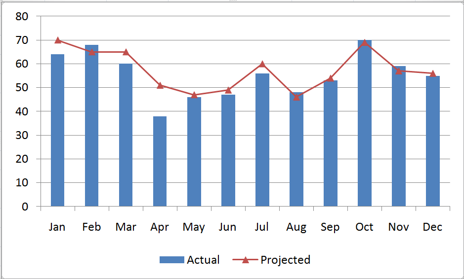
A combination chart in Excel is not a single chart type. Rather, you create combination charts by combining two or more complementary chart types. The most common combination is a Column type for one series and a Line type chart for the second series. Combination Charts, in general, make it easier to spot or highlight the trends in your data.

Combination Chart

Excel Combination Chart

 Creating a Combination Chart

  1. Create a standard chart for your data.
  2. Select one series and then choose a different chart type for that series.
  3. Make formatting choices as necessary.

Adding a Secondary Axis for Data

When you are comparing data series that have a wide “gap” between them – e.g. comparing actual sales in a month (large number) – to Profit % in each month (small number), you will want to create a Secondary Vertical (Value) Axis in your Combination Chart.

Begin by selecting the series that you want to plot and Right Mouse Click to Format the Series on a Secondary Vertical Axis. I recommend that you add in Axis Titles for both the Primary and Secondary Vertical Axes.

Formatting Charts in Excel 2007 and 2010

Charting in Excel – beginning with Version 2007 – now offers quite a few professional graphic design elements. In this video lesson, I show you how to customize the presentation of your graphical image. You can make these changes with just a few mouse clicks! It is definitely worthwhile to learn how to improve the visual impact that your Combination Charts make.

Learn how to “Master Excel in Minutes – Not Months!”

Follow this link to watch this Excel Video in High Definition, Full Screen Mode on my YouTube Channel – DannyRocksExcels

Subscribe to or watch my – free – video podcast on iTunes.

How to Create a Combination Chart in Excel

What is a Combination Chart? When do I use one? Why do I use one?

  1. What: A combination chart uses two different chart types in the same graphic representation of your data.
  2. When: There is a large value gap between one data series and the other data series.
  3. Why: To reveal the relationships in your data that may not be apparent with a traditional chart or by merely examining the data.

In this short video lesson, I will demonstrate “How” to transform a traditional column chart into a Combination Chart that reveals an interesting data relationship.

Here are the steps to follow in this Excel Video Lesson:

  1. Start with a standard Excel Chart – Here we used the F11 Key to create a Column Chart in a separate worksheet.
  2. Notice the wide gap between the two data series. Click on one of the series columns (in this case “Dollars”) and on the Chart Toolbar select the “Line” chart type.
  3. A wide gap in values remains between the two series. With the “Dollars” series selected, choose Format Series on the Toolbar. Click the Axis Tab and select “Plot Series on Secondary Axis.”
  4. Format the chart to suit your needs. In this example, we change the color of the Plot Area and add Text to a “Call out” shape on the chart.

Find the Excel Video Lesson that you want. Index of all Excel Topics

News! My DVD, “The 50 Best Tips for Excel 2007” is now available to purchase. I invite you to visit my online bookstore for more details.

Related Videos