How to Create Custom Views of a Worksheet in Excel

Custom Views in Excel

Custom Excel Views

This is Part 2 in my series of video tutorials demonstrating the Commands found on the View Tab of the Excel Ribbon. Building on the concepts that I demonstrated in Part 1 (“How to Freeze Row and Column Labels While Scrolling in Excel”), I now show you how to save these settings as a Custom View.

Create a Custom View in Excel

  1. Display the settings that you wish to save as a Custom View – e.g. Changing the ZOOM Level of Magnification, Freezing Rows or Columns, etc.
  2. From the View Tab on the Ribbon, choose the Custom Views Command.
  3. In Custom Views Dialog Box, click Add; Give your View a Name and Click OK.
  4. Remember to Save your Excel Workbook. To test your custom view, I recommend that you revert to your normal or default view and save that version. Then close the workbook and reopen it. Now, it will display the last view displayed when you saved the workbook. Click on the Custom Views Command and select the Custom View that you recently added; the Custom Settings will now display.
  5. Add – and Save – additional Custom Views.

Custom Views are Worksheet Level Views

When you create a Custom View, it only applies to the Excel Worksheet where you created it. In fact, while you “Show” a Custom View, all other Worksheets in the Active Workbook are NOT available.

Excel Tables and Custom Views

 There is one “gotcha” with Custom Views. If you have formatted a data set as an Excel Table on ANY worksheet in the workbook, ALL Custom Views are blocked out. Watch  this video to see how to “work around” this roadblock.

Online Shopping at The Company Rocks

I invite you to visit my secure online shopping website – http://shop.thecompanyrocks.com – to preview all of the resources that I offer you.

Watch Tutorial in High Definition

Follow this link to view this Excel Tutorial in High Definition on my YouTube Channel – DannyRocksExcels

Play Video Now


How to Outline an Excel Worksheet

Many Excel worksheets – e.g. Budgets and Sales Reports – can be improved by applying an Outline. With an Outline, you can switch your focus between looking at the “big picture” and examining the details. An outline is especially useful when you are presenting numbers “interactively.” For example, when you are using a Projector and Screen to present Quarterly Sales Results during a meeting.

Outline Commands
Outline Commands

If you have set up your Excel worksheet in a “hierarchical” structure – SUMs at the bottom and to the right of each category, creating an outline is simple:

Create the Outline

  • Select a single cell in the worksheet.
  • On the Data Tab of the Ribbon (Excel 2007) go to Group – Auto Outline.
  • You now see the Outline Symbols “+ and -” above each column and to the left of each row. Depending on your data, you will also see numbers that represent the “level” of Outlining available.

Examine the Formulas

When a client sends me an Excel worksheet, one of the first steps that I take is to find all of the cells that contain formulas. A quick way to do this is with the F5 Keyboard Shortcut. This opens the “Go To” Dialog Box. Choose “Special” and then select “Formulas.” Now, all of the cells that contain Formulas are highlighted. If everything is correctly organized, then I apply the “Auto Outline” command to the worksheet.

Keyboard Shortcuts

Use the Ctrl + 8 keyboard shortcut to “toggle” between Hiding and Displaying the Outline Symbols. This is a great tip to learn – you still have the Outline, but your screen looks cleaner. And … I guarantee that several people in your audience will ask you “How did you do that?”

Custom Views

During the video lesson, I also show you how and why to apply Custom Views to your Outlines. A Custom View allows you to quickly display a different perspectives of your data. Set them up in advance – it is almost like having a PowerPoint slide presentation inside your Excel worksheet outline!

You can watch this Excel video lesson in High Definition, Full Screen mode on my DannyRocksExcels YouTube channel.

Learn how to “Master Excel in Minutes – Not Months!”

How to Filter Excel Data and Save Custom Views

With an Excel data set, you rarely want to view all of the records – hundreds or thousands of records. Rather, you want to view a subset of the data – e.g. Sales of Laptop Computers in June sold by Bob. To do this, you create and apply filters. A filter is similar to a query – you are asking a question and getting the answer – information – from your data. If this is a question that you ask frequently, you can save the filter as a Custom View.

Filter Types in Excel

Filter Types

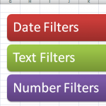
In Excel 2007, filtering has been greatly improved with the introduction of Date Filters, Text Filters and Number Filters. Now it is easy to find the sales for “last week,” or the invoices that will be due “next month,” etc. These new filter types – also available in Access 2007 – allow you get better information quicker from your data set.

Top 10 and Above Average Filters

In this lesson, I also demonstrate how to use the “Top 10” filter. You can also use the new “Above Average” and “Below Average” number filters to quickly find your best performers.

Create Custom Views

There is one “frustration” with Custom Views: If you use Tables in Excel 2007, you cannot use a Custom View. In fact, all Custom Views are disabled if you have a Table on any worksheet in your Excel Workbook.

You can learn more about filtering in Excel – click here to watch my video on Using Advanced Filters in Excel.

Want to watch this video in High Definition, Full-screen Mode? Click here to go to my DannyRocksExcels Channel on YouTube.

View my Video Podcast on iTunes. Click here to go to my iTunes Video Podcast, “Danny Rocks Tips and Timesavers.”

Learn how to “Master Excel in Minutes – Not Months!”