In this tutorial – the second in my series explaining how a worksheet, that my accountant friend Alan Friedman created, works – I focus on improving the formatting for the column labels and other descriptive text.
Wrap Text for Labels
In my experience, I find that many accountants and other financial managers have not mastered the basics of formatting an Excel Worksheet. It seems that they are still using “old fashioned IBM typewriter tricks” when it comes time to create the labels for the columns of data in their spreadsheet.
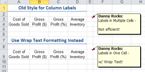
Case in Point: Using two or more vertical cells to type “Cost of” (Return key on Computer) “Goods Sold.” This “old fashioned” process will lead to multiple problems. For example, improper sorting and filtering of data.
In this tutorial, I demonstrate how to use the Wrap Text command to format a single-cell text label. You will also learn how to use the Keyboard Shortcut Alt + Enter to control where your text “breaks” when wrapping text.
Merge Cells Across Columns
When you have a long, descriptive text – e.g. Your Company Name – it is best to type this into a single cell and then use the Merge Cells Command. Now, when you double-click between Column Letters to automatically expand the width of a column, only the “um-merged” labels in the column are extended in width.
Additional Resources for Tutorial
You can learn “The 50 Best Tips for Excel 2007” on my DVD-ROM. Visit – http://shop.thecompanyrocks.com/50-best-tips-for-excel-2007/ – to learn more about this.
Click on this link to download the Excel Worksheet – created by Alan Friedman – that I use in this lesson.
Watch Tutorial in High Definition
Follow this link to watch this tutorial in High Definition on my YouTube Channel – DannyRocksExcels

