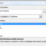
Database Functions include DSUM, DAVERAGE, DCOUNT. They are easy to use. You can use them with your Excel Tables and Lists. You use Database Functions to return the results (Sum, Average, Count, etc.) that you get from a Filter – or in this case, The Criteria.
Database Function Arguments
Each Database Function uses the same three required arguments:
-
- Database. The Range that begins with your Data Set Labels and includes each column and each row in the database range. I prefer to use a “Named Range” for this argument.
- Field. The reference to the Field Label for the field that you wish to calculate (Sum, Count, Average, etc.) There are three ways to refer to this label: (Click on the cell with the label, use a column reference number (1,2,3, etc.) counting from Left to Right, type the “Label Name” inside ” ” quotation marks.
- Criteria. The Criteria Range that includes the Column Label for the criteria and the cells that contain the values or formulas you are using as your criteria.
It takes only a few minutes to set up your “Excel Dashboard” for the Criteria Range and your Results (e.g., the sum of the values in the field that match your criteria.) Change a value in your criteria and your results update automatically.
Filtering Data in Excel
If you use a structured data set in Excel, you probably use AutoFilters or Advanced Filters. Use Database Functions to “capture” the totals, averages, and counts of those queries.
If you need to review or learn how to apply Filters to data in Excel, watch these two lessons:
- How to Apply Criteria for Advanced Filters in Excel
- How to Filter Data and Use a Custom View in Excel
Click here to watch this video in High Definition at DannyRocksExcels on YouTube.
I invite you to shop for my DVD-ROM, “The 50 Best Tips for Excel 2007.” Click here to open a secure shopping cart.
Learn how to “Master Excel in Minutes – Not Months!”


