How a Single Blank Cell Affects an Excel Pivot Table Report

As you will see in this Excel Video Tutorial, having a single blank cell in a data set will greatly affect how Excel Functions and Pivot Tables are designed and calculated.

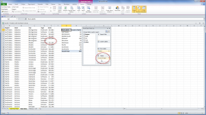
Single Blank Cell in Data

Single Blank Cell in Data

Imagine, how a single blank cell, in a field of 848 records, can change the way your Pivot Table views the data type (text vs. the expected numeric data type) and subtotal function (Count vs. the expected SUM function).

Seeing is believing!

Preventing a Blank Cell from “Creeping into” your data set

Use the Keyboard Shortcut Ctrl + Down Directional Arrow to go to the last cell that contains data in a column. This is a great way to isolate “stray” blank cells that will have a great impact on your Pivot Tables and other calculations in Excel.

Also, in Excel 2007 and Excel 2010, look for where a “numeric” field is placed by default. A single blank cell will cause an (intended) numeric field to be placed in the Row (text) labels area. Even dragging this field into the VALUES Drop zone does not solve the problem because the COUNT Function will be used to Subtotal this field. This is a “disaster waiting to happen!”

Introducing My Extended Length Excel Video Recordings

This is my opportunity to introduce you to my new, extended-length (one-hour +) Excel Video Tutorials that you can download for only US $9.95!

Here is the link that gives you more information about this exciting new service:

http://www.thecompanyrocks.com/pivot-table-tutorial-videos-to-download-practice-files-instructional-manual-included/

I offer you multiple options:

Let me know what you think!

Let me know which topics you would like me to record for you to download.

Send me an email with your comments and suggestions: danny@thecompanyrocks.com

Watch This Video in High Definition

Follow this link to view this Excel Tutorial in High Definition on my YouTube Channel – DannyRocksExcels

How to Maintain Accurate Subtotals When Your Data Set Expands in Size

Subtotal in Excel 2010 Table

Subtotal in Excel 2010 Table

This is Part 2 of my series of video tutorials demonstrating how to use the SUBTOTAL Function in Excel.

  • In Part 1, I showed you the value of using the Subtotal Function to summarize the results of applying a Data Filter to a range of cells.
  • In this part, I show you how to use an Excel 2007 or Excel 2010 Table to ensure that your Subtotal Formulas are automatically updated when you append records or add additional fields to your original data set.

I strongly recommend basing Filtered Lists and Pivot Tables on an Excel Table (in Excel 2007 or 2010) or an Excel List in Excel 2003. This way, any formulas, filters and references that you make will be automatically updated when you append additional records or otherwise change the structure of your data set.

Function Numbers 101 through 111

Notice that when you “toggle on” the Total Row for a Table or List that Excel uses this formula = SUBTOTAL(109, Table1, [Sales]). Function 109 will use the SUM Function(109) to total the values in the “Sales” field ([Sales]) of a Table named “Table1.” These Function Numbers + 100 were introduced in Excel 2003 and the are automatically applied whenever you are using a Total Row in an Excel Table.

I think that you will learn some cool tricks in this lesson. Let me know what you think!

Watch This Video in High Definition

Click on this link to watch this video tutorial in High Definition, Full Screen Mode on my YouTube Channel – DannyRocksExcels.

Invitation to Visit My New Online Shopping Site

I invite you to visit my new, secure online shopping website – http://shop.thecompanyrocks.com

Once there, you can get my best-selling DVD-ROM, “The 50 Best Tips for Excel 2007”

Functions to Analyze Loan Payments in Excel

Loan Payment Functions

Loan Payment Functions

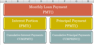
When you use the PMT Function in Excel, the result is the amount of money that you will pay each period (usually monthly) until the loan is repaid. When you want to know how much of each payment is an interest charge, you use the IPMT Function. And,to find the amount that goes towards reducing the principal on your loan, you use the PPMT Function.

Cumulative Payments

Two other functions are helpful in analyzing your loan payments. When you want to see the Cumulative amount of Interest (CUMIPMT Function) that you paid between two periods – e.g. Starting with payment 1  and ending with payment 12. You use the CUMPRINC Function to total the amount of your loan payments that went towards reducing the principal on your loan between any two periods.

Absolute and Relative Cell References

As you will see in the video, I use a combination of Absolute Cell References (e.g. $A$4) and Relative Cell References (e.g. A4) in these formulas. An Absolute Cell Reference means that cell will “remain in place” when the formula is copied down or across to other cells. In this example, I have my Loan Information (Amount to borrow, Interest Rate, etc.) at the top of the spreadsheet. Almost all references to these cells in formulas is Absolute.

Function Arguments Dialog Box

I almost always use the Function Arguments Dialog Box when I am creating my formulas. I use the Keyboard Shortcut, Ctrl + A at this point in the formula – “=PMT(” to activate the dialog box. The advantages of using the Function Arguments Dialog Box are:

  • Explanation of both the function and each “argument” in the function
  • Ensures arguments are answered in the proper sequence
  • Ensures that all “required” arguments (Argument Labels are in Bold)
  • Evaluates the result of each “intermediate” calculation – to the right of each argument

This is the first of several Excel Video Lessons that I am creating to demonstrate how to perform Financial Calculations. Let me know what you think or send me your questions to answer. You can add a comment below this post.

Watch This Video in High Definition on YouTube

Follow this link you view this Excel Video on my YouTube Channel – DannyRocksExcels

Download Excel Workbook

Follow this link to download the Excel Workbook I used in this lesson.

Subscribe to My Video Podcast

I invite you to receive an automatic notice – via email – whenever I publish a new Excel Video Lesson. Follow this link to find out the details. The subscription is free; you do not need to provide and personal information beyond your email address; and you can cancel at any time – no questions asked!

How to Use Conditional Formatting to Compare Two Excel Lists

Clients and viewers frequently ask me to help them to compare two differeny lists in Excel. They want to find – or highlight – the values that are different in each list. For example, which customers appear in the 1st list but NOT in the 2nd list. So, I created this video lesson to demonstrate how to do this with Conditional Formatting.

In an earlier Excel Video Lesson, I demonstrated how to compare two Excel lists using either the MATCH() Function or the VLOOKUP() Function.

Conditional Formatting Rule

Conditional Formatting Rule

Use Conditional Formatting

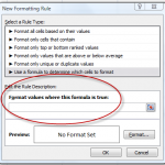
I demonstrate how to use Conditional Formatting to Highlight the Cell Values that are different when you compare two Excel Lists. I will use a “New Rule with a Formula” that must return the answer TRUE, to trigger the special formatting.

In Conditional Formatting, you first establish a “condition” that can be answered as either TRUE or FALSE. Then, for those cells where the answer to the condition is TRUE. the special “cell formatting” that you chose will apply.

In this lesson we will be using this Formula: =COUNTIF(List 2, 1st cell in List 1) = 0.

Steps to follow:

  1. Select the cells that you want the Conditional Formatting to apply to- in our example List 1.
  2. On the Home Tab of the Ribbon, click the Conditional Formatting arrow and select New Rule.
  3. Select New Rule – “Use a Formula to determine which cells to format.”
  4. Enter the formula – e.g. =COUNTIF(Range, Criteria) = 0 where the “Range” is the list of values in List 2 (Absolute Reference) and the “Criteria” is the 1st cell reference in List 1 (Relative Reference).
  5. Choose the Format for the cells when the condition is met – the result is TRUE. In this example, I choose to “FILL” the cells with a Blue background color.

Want to watch this video in High Definition, Full-Screen Mode? Click here to go to my YouTube Channel, DannyRocksExcels

Learn to “Master Excel in Minutes – Not Months!”

How to Use the SUMPRODUCT Function in Excel

In my experience, most Excel users are unfamiliar with the SUMPRODUCT Function. So let me give you two reasons to watch this short (5 minutes, 22 seconds) video lesson to learn how – any why – to use SUMPRODUCT:

  1. The SUMPRODUCT Function will speed up your calculations in Excel – get results with one step. With SUMPRODUCT() you can avoid several intermediary calculations.
  2. With SUMPRODUCT, you may be able to trim the size of your Excel worksheet. You may not need as many columns (fields) as you think to get the result that you need!

In this lesson, I show you how to calculate the Total Value of the Inventory (for a fictional company) with one formula!

50 Best Tips for Excel 2007

Excel Tips

Key Points Coverered

While the SUM Function “Adds Up” the values in the Arguments, the PRODUCT Function “Multiplies” the values in its Arguments.

  • Using “Arrays” in SUMPRODUCTS. In Excel 2007, you can use up to 255 Arrays! The key point is that all Arrays must be the same size and shape. For example, if the 1st arry in the Arguments is 15 rows in one vertical column, then all of the subsequent Arrays must be 15 rows in one vertical column.
  • I find that Creating – and Using – Names Cell Ranges for the Arrays will speed up writing the SUMPRODUCT formula.

I have decided to present the SUMPRODUCT Function in two lessons – so click on the sequel to see other uses for this function!

Click here to watch the 2nd video lesson on how to use the SUMPRODUCT Function in Excel.

You can watch this Excel Training Video Lesson in High Definition, Full Screen Mode on my YouTube Channel – DannyRocksExcels

You can learn how to “Master Excel in Minutes – Not Months!”

Use the Choose Function in Excel to Quickly Lookup a Value

The CHOOSE Function in Excel is an incredibly useful – albeit, relatively unknown – tool to use when you need to look up a Value in a list. In Excel 2007, you can now use CHOOSE to return up to 254 different Values in a list! (In Excel 2003, the limit is 29 values.)

Here is the Syntax: =CHOOSE(Index_Num, Value1, Value2…) where the Index_Num is a positive serial number between 1 and 254 (In Excel 2007)

In this lesson, I first demonstrate how to look up a “label” (January, February, etc.) for a cell that contains a “Number” for the month (1,2,3, etc).

Rather than struggle with “nested IF()statements,” use the CHOOSE Function when you need to return a value for any number between 1 and 254 – it is so much easier!

Click here to watch this Excel Lesson on YouTube in High Definition Full Screen Mode.

Learn how to “Master Excel in Minutes – Not Minutes!”

Create Interactive Excel Forms Using Option Button Controls

This is the third in my series of video lessons that show you how to add Form Controls to an Excel worksheet. Option Buttons, inside a Group Box, are a great way to make your forms “interactive” – to give your end-user multiple options. For example, a choice of shipping methods for their order. Or, to see how different “down payment” options effect their mortgage payments.

The key to understanding how Excel Form Controls operate is to see how the value in the “cell link” changes when you choose an option. The cell link for an Option Button translates a “text expression” into a numeric value. For example, “Surface” translates to “1” for a shipping option.

In this Excel Training Video, I introduce the =CHOOSE() Function. It is rare that I find a client who has ever used this function. Once you see how useful it is, you will start to use it instead of struggling through multiple =IF() Functions. It is really a great “hidden gem” of an Excel Function!

Click on this link to go to my Archive of Excel Video Lessons on Forms. 

You can also find additional groups of related videos by selecting a “Category” from the drop-down menu on the right side bar of any page on my website.

Learn how to “Master Excel in Minutes – Not Months!”

Tell Excel 2007 Not to Display a Formula Error in a Cell

Excel 2007 introduces a brand new Function – the =IFERROR() Function which is a great way to “hide” any potential Formula Error Messages from displaying. You know these error messages – #DIV/0!, #NULL – They are ugly to look at and they can harm your professional reputation.

Watch how you can use =IFERROR() in Excel 2007. Or, if you are using Excel 2003, I show you how to accomplish the same goal but with a few more steps using the =ISERROR() Function nested inside an =IF() Function.

(Note: This is a repost. I now have a Podcast on iTunes and I need to feed this video to the iTunes Store.)

You can subscribe to my iTunes Podcast by clicking on this link.

Learn how to “Master Excel in Minutes – Not Months!”

Trust Your Sources but Verify Your Data’s Accuracy

You may be familiar with the expression, “Trust but Verify!” President Reagan used this phrase when referring to the Soviet Union’s agreement to disarm their missiles. It is also a good approach to follow when you receive Excel data from someone else:

  1. Never open up a data file unless you trust the source.
  2. Never make a decision on the data until you verify the accuracy of the formulas and the structure of the spreadsheet.

In this Excel Video Lesson, I demonstrate how to use the GoTo Special Dialog box to verify the accuracy of your data.

Here are the steps to follow in this lesson:

  1. Choose Edit – GoTo – Special – Formulas to highlight all of the cells containing formulas in the worksheet.
  2. The Keyboard Shortcuts for “GoTo” are Ctrl+G or the F5 Key.
  3. In the “Special” dialog box, you can also choose “Constants.” This may make it easier to spot the cells that are “hard-coded” with a constant value when they should contain a formula.
  4. You can narrow your selection to “Text,” “Logical,” Numeric,” etc. formulas.
  5. Use the Ctrl+~ (Tilde) Shortcut to show the actual formulas in your worksheet.

NEW! Download the Practice File Used in This Excel Training Video

Find the Excel Video Lesson that you want – Index to all Excel Topics

News! My DVD, “The 50 Best Tips for Excel 2007” is now availabe to purchase. I invite you to visit my online bookstore for more details.

Related Videos

Excel’s QuickSum Calculator – Get Results Without Writing a Function

MS Excel 2003 has a great feature – The QuickSum Calculator – but you have to know where to find it. It is on the Status Bar – that area at the lower right of your screen. Simply select at least two data cells. They can be contiguous or non-contiguous. But remember where to look for the QuickSum Calculator  – it is on the Status Bar.

Want to change the function? It simple! Just right-click on the name of the Function. You can choose Average, Count, Count Numbers, Min or Max – Excel’s most common Functions.

This is a great way to perform an Ad-hoc Query. I recommend that you use this for spreadsheets with Subtotals. Watch this short video lesson to see how this works – and how you can save time!

Find the Excel Video Lesson that you want – Index of all Excel Topics

News! My DVD, “The 50 Best Tips for Excel 2007” is now availabe to purchase. I invite you to visit my online bookstore for more details.