How to Use Keyboard Shortcuts in Excel to Control Basic File Operations

Excel 2007 File Operations

Excel 2007 File Operations

If you have recently upgraded to either Excel 2007 or Excel 2010, you REALLY NEED to master the Keyboard Shortcuts that I present in this lesson!

Many Excel veterans who upgrade, tell me that they initially felt “lost” with the new user interface. Some of my clients called me in a panic because they didn’t know where to look to Print their work or to open a document. If you know how to use the Keyboard Shortcuts that I present in this lesson, you will never be at a loss. As an added bonus, these Keyboard Shortcuts work with ALL Microsoft Office programs and also for most Windows-based programs.

The “N-O-W-S” Keyboard Shortcuts

I use this acronym – NOWS – to remember the keyboard shortcuts to Open, Close and Save Documents in MS Office programs. Use Ctrl + W to Close the active worksheet.

In this video tutorial, I also show you when NOT to use Keyboard Shortcuts! There are many times when you need to access the full file menu selection.

Keyboard Shortcut for Print Preview

Use Ctrl + F2 to open up the Print Preview pane. Use the “Esc” key to Exit Print Preview.

Download My Chart of Popular Keyboard Shortcuts as a PDF

Follow this link to go to the web page where I store my Keyboard Shortcut Charts and other download-able content.

These Keyboard Shortcuts work for all versions of Excel. So far, I have found only one Keyboard Shortcut that is different when used in Excel 2007 / 2010 than in Excel 2003.

More Video Tutorials for Keyboard Shortcuts

This is the first in a series of video tutorials that I have planned. Each video will focus on the Keyboard Shortcuts you can use to perform a specific task – e.g. Formatting Cells, Inserting and Deleting, etc. My plan is to post one new video in this series per week.

Watch Video Tutorial in High Definition Mode

Follow this link to view this video tutorial in High Definition on my YouTube Channel – DannyRocksExcels


Write a Custom Excel Function to Link Worksheet Tab Name to a Cell

Custom Functions in Excel

Custom Excel Functions

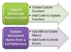
In response to many viewer requests, I am creating a two-part series of video tutorials that show you how to create links between the name of an Excel Worksheet Tab and a cell on that worksheet.

Here, in Part One, I demonstrate how to write a Custom Excel Function to capture the name of the worksheet tab in a cell.

Write Custom Excel Functions

You write Custom Excel Functions in the Visual Basic Editor. One way to open the Visual Basic Editor is to use the keyboard shortcut Alt + F11. Here are the elements that I use in this lesson:

  • Open the Project Explorer Pane (Keyboard Shortcut Ctrl + R).
  • Insert a Module to contain the VBA Code that you write for your Custom Function
  • Open the Code Pane (Keyboard Shortcut F7).

Write the Code for the Custom Function

In its simplest form, this is all of the code that you need for this Custom Excel Function:

Function SHEETNAME2() As String
SHEETNAME2 = Application.Caller. Parent.Name
End Function


That’s it!

Automatically Update Results of Custom Functions

A major difference between Custom Functions that you write and Excel’s Built-in Functions is that by default, the result of a Custom Function does not automatically update when values or references change. If you want your Custom Function to automatically update whenever the worksheet changes, add this line of code to your Custom Function in the Module:

Application.Volatile True

Source for this Code

I found the code for this Custom Excel Function in John Walkenbach’s Book, “Excel 2007 Formulas. He is an Excel Expert and I admire his writing style. You can check out his reources at this site:

http://spreadsheetpage.com/

Watch this Video in High Definition on YouTube

Click on this link to view this Excel Tutorial on my YouTube Channel – DannyRocksExcels.

Watch Part 2 of This Series

Here is the link to Part 2 in this Series. In this lesson I show you how to write an Excel Macro in VBA to update the Name of the Worksheet Tab based upon the value in a cell on the worksheet.

New Keyboard Shortcuts for Paste Special in Excel 2010

Content Key on Keyboard

Content Key on Keyboard

In Excel 2010, you can now use special keyboard shortcuts to control your Paste Special Options – e.g. Paste Values Only, Transpose, Paste Link, Paste Formatting, etc.).  There is a new technique to learn, however, before you can become proficient with these keyboard shortcuts in Excel 2010. Let me demonstrate.

Live Preview for Paste Special in Excel 2010

In my previous video tutorial, I demonstrated how to take advantage of this great new feature – “Live Preview for Pasting” – in Excel 2010. Click here to watch that video.

Two Ways to Use Keyboard Shortcuts to Paste Special in Excel 2010

  1. Press and Release the Ctrl Key, then press the “letter key” for the shortcut.
  2. Press the “Context Key” on your keyboard (to the right of the Space-bar; between the Alt & Ctrl keys) and then press the “letter key” for the shortcut.

Each of these techniques is easier to explain through a video demonstration than to write out the instructions. So, I encourage you to watch my video if you want to learn these new techniques for Excel 2010!

Learn More Paste Special Options

Main Menu Essential Skills for Excel

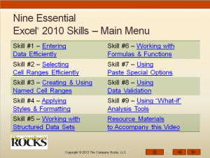
Main Menu for “9 Essential Excel Skills”

On my latest DVD-ROM, “Nine Essential Skills for Excel 2010,” I go into greater detail about the many ways that you can use Paste Special. This IS one of the 9 Essential Skills that I have identified. Follow this link to learn more about the 4 hour training video. The DVD-ROM includes 25 individual video tutorials, a 29-page instructional manual,  and the Excel 2010 Practice Files that I used while filming the videos.

Learn about all of the training resources that I offer at my secure online shopping website – http://shop.thecompanyrocks.com

Watch Video in High Definition on YouTube

Follow this link to watch this video tutorial in High Definition on my YouTube Channel – DannyRocksExcels.

Free Video Recording of Excel Keyboard Shortcuts to Download

I have just published a 50 Minute Video Recording on which I demonstrate the most popular Keyboard Shortcuts for Excel. The great news – for you – is that you can download this video recording for FREE! If you prefer to view this online, you can do so – for FREE!

Download My Excel Workbooks

Download my Workbooks

Download Excel Workbooks

In addition, I have published the Excel Workbooks, Adobe PDFs and PowerPoint files that I use during this 50 minute video online. You can access them – for FREE!

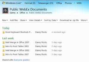
I store them as “public documents” for you to download on my “Sky Drive” at Windows Live! Here is the direct link:

http://cid-644f2f857aa6afdc.office.live.com/browse.aspx/Public%20WebEx%20Documents/Excel%20Keyboard%20Shortcuts%20Part%201

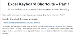
In order to access these files, you will need a “free” Windows Live account (First Name, Last Name, email address). You can also use your HotMail account to login.

My Extended Length Video Recordings on WebEx

I have recently began to publish “extended length” video recordings at http://thecompanyrocks.webex.com – This 50 Minute video is my 5th recording on the site. I offer it to you “free of charge.” However, you must register (fitst name, last name, email address) with WebEx by Cisco before you can download the recording or view the recording online.

In this format, I can offer “specialized instruction” for Excel Pivot Tables, Macros, Public Speaking Courses, etc. I can also offer instruction in older (Excel 2003) and newer (Excel 2010) programs. In addition, I can create a specialized recording “just for you.” Contact me to learn about how to organize this!

Landing Page for More Information

Links for Downloads

Information about Links and Downloads

Rather than repeat what I have already written, here is the link to the special Landing Page that I have created for this 50 minute video recording. On the Landing Page, I have included all of the direct links to the download pages for the video, the Excel files, PowerPoints and Adobe Acrobat documents that I used on this recording.

I invite you to view or download these new resources that I have made available. When you have a chance send me your comments, questions and suggestions for future recordings!

Danny Rocks

The Company Rocks

Watch This Video Lesson in High Definition

Click here to go to my DannyRocksExcels YouTube Channel where you can view this tutorial in High Definition.

Get My New Popular Keyboard Shortcuts for Excel Chart – It’s Free When You Register

Click the link below to download my chart of Excel Keyboard Shortcuts as a PDF:
Excel Keyboard Shortcuts

Preview Excel Keyboard Shortcuts

 Hello and Welcome – to my new “Members Only” section of The Company Rocks website! 

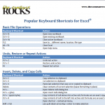
I just published a new five-page Chart – “Popular Keyboard Shortcuts for Excel.” It is free for you to download as a PDF. 

This, along with additional content, will soon be inlcuded in my new “Exclusive Membership Content” area on my website. 

My Exclusive Membership Site is not quite ready to launch. So, I am offering this chart for you to download as a PDF from this post. 

To get this chart, click on this link –  

CR – Updated Chart of Popular Excel Keyboard Shortcuts 

New! Download My Free 50 Minute Video Recording Demonstrating Excel Keyboard Shortcuts

Click this link to learn how you can download my new “extended length” video recording. It is “free of charge!”

I am proud of the way my Excel Keyboard Shortcuts Chart turned out – and I think that you will get a lot of value out of this free resource. I organized the Keyboard Shortcuts by the following Tasks:

Excel Keyboard Shortcuts

  • Basic File Operations
  • Undo, Restore or Repeat Actions
  • Insert, Delete, and Copy Cells
  • Edit Data
  • Show / Hide Columns and Rows
  • Select Contiguous Cells
  • Navigate Within a Worksheet
  • Navigate Between Workbooks
  • Find, Replace, and Go To
  • Enter Data
  • Work with Cell Comments
  • Work with Names for Cells and Ranges
  • Work with Formulas and Functions
  • Work with Formula Precedent and Dependent Cells
  • Print Worksheet
  • Formatting Cells and Text
  • Work with Subtotals and Outlines
  • Work with Tables, Lists, and Filters
  • Work with Charts
  • Work with Excel Windows and Open Applications

So, as you can see, this is a comprehensive – but not exhaustive – list of the best Keyboard Shortcuts for Excel. I took care to ensure that these Keyboard Shortcuts will work for all versions of Excel from 2003 through version 2010. 

The 50 Best Tips

The 50 Best Tips Series

I have several video lessons that cover keyboard shortcuts on my DVD-ROM, “The 50 Best Tips for Excel 2007.” It is a best-seller and it is now on sale! Use Coupon SAVE-20-PCT at checkout and save 20% on any puchase at my online store. Click here to open a secure shopping cart

And let me know your thoughts on my Excel Keyboard Shortcut Chart. Do you have a favorite Keyboard Shortcut that you want to share with our readers? Add your comments below.

Learn how to “Master Excel in Minutes – Not Months!”

How to Outline an Excel Worksheet

Many Excel worksheets – e.g. Budgets and Sales Reports – can be improved by applying an Outline. With an Outline, you can switch your focus between looking at the “big picture” and examining the details. An outline is especially useful when you are presenting numbers “interactively.” For example, when you are using a Projector and Screen to present Quarterly Sales Results during a meeting.

Outline Commands
Outline Commands

If you have set up your Excel worksheet in a “hierarchical” structure – SUMs at the bottom and to the right of each category, creating an outline is simple:

Create the Outline

  • Select a single cell in the worksheet.
  • On the Data Tab of the Ribbon (Excel 2007) go to Group – Auto Outline.
  • You now see the Outline Symbols “+ and -” above each column and to the left of each row. Depending on your data, you will also see numbers that represent the “level” of Outlining available.

Examine the Formulas

When a client sends me an Excel worksheet, one of the first steps that I take is to find all of the cells that contain formulas. A quick way to do this is with the F5 Keyboard Shortcut. This opens the “Go To” Dialog Box. Choose “Special” and then select “Formulas.” Now, all of the cells that contain Formulas are highlighted. If everything is correctly organized, then I apply the “Auto Outline” command to the worksheet.

Keyboard Shortcuts

Use the Ctrl + 8 keyboard shortcut to “toggle” between Hiding and Displaying the Outline Symbols. This is a great tip to learn – you still have the Outline, but your screen looks cleaner. And … I guarantee that several people in your audience will ask you “How did you do that?”

Custom Views

During the video lesson, I also show you how and why to apply Custom Views to your Outlines. A Custom View allows you to quickly display a different perspectives of your data. Set them up in advance – it is almost like having a PowerPoint slide presentation inside your Excel worksheet outline!

You can watch this Excel video lesson in High Definition, Full Screen mode on my DannyRocksExcels YouTube channel.

Learn how to “Master Excel in Minutes – Not Months!”

Learn How to Use Date Functions in Excel

Excel has a group of functions that help you to calculate dates. For example, the number of days between two dates or the date on which an invoice will be payable.

This is the second in my series of lessons where I demonstrate how to enter and calculate dates and times in Excel. Here is the link to part one.

Excel Tip List

Excel DVD Tips

The date functions that I demonstrate on this video are:

  • TODAY()
  • NOW()
  • DATE()
  • DATEVALUE()
  • WORKDAY()
  • NETWORKDAYS()
  • EOMONTH()

The last three date functions require you to activate the Analysis ToolPak Add-in. You will also learn some valuable and time saving keyboard shortcuts.

You can watch this video in High Definition, Full Screen Mode on my YouTube Channel – DannyRocksExcels

Learn how to “Master Excel in Minutes – Not Months!”

How to Work with Dates in Excel

The majority of the questions that I receive from viewers center on how to use and format DATES & TIMES in Excel. So, I have decided to create a series of lessons to show you how to work with dates and times in Excel.  This is part one in a continuing series of free Excel Video Training Lessons.

50 Best Tips for Excel 2007

Excel Tips

Learn How to Work with Dates

  • Use a Keyboard Shortcut to enter the current date in a cell – to “time stamp” the date.
  • Use the TODAY() Function to enter a “dynamic” date function in a cell – so that your date always reflects the current date.
  • Distinguish between how Excel “stores” a date – as a serial number – and how Excel formats a date – how you choose to format a date.
  • Tell if a date was entered correctly – as a number – or incorrectly – as “text” by seeing how it is aligned in the cell (right or left).
  • See why a fraction could be recognized as a date – and how to correct this “got’cha” step!
  • How to create a series of dates in your spreadsheet.

In my experience, the majority of “Excel problems” are based around incorrect date and time entries. So, whether you are new to Excel or a veteran who gets frustrated with Time and Date calculations, this lesson is for you.

If nothing else, you will pick up some great Keyboard Shortcuts in this lesson!

Follow this link to watch this video in High Definition, Full Screen Mode on my YouTube Channel – DannyRocksExcels

Learn how to “Master Excel in Minutes – Not Months!”

Use the SUMPRODUCT Function to Total Lists Using Multiple Criteria

In Excel 2007 and Excel 2010 you can use the new SUMIFS Function to total a list using multiple criteria. This is a great new feature!

But … what if you are using Excel 2003 or earlier? Or, if you collaborate with colleagues and clients who use older versions of Excel – how can you use multiple criteria to select the records that you want to Sum? You can use the SUMPRODUCT Function as I demonstrate in this video lesson.

The 50 Best Tips

The 50 Best Tips Series

Key Concepts

  • Create – and use – Named Cell References for Ranges / Arrays in your formulas
  • Use the Function Arguments Dialog Box – Use the keyboard shortcut Ctrl + A to bring this up
  • Use the F3 Keyboard Shortcut to bring up the Named Ranges List
  • In this lesson, use () to enclose each Array Argument
  • In this lesson, use * to substitute for the , to separate each Array in the formula (Edit this in the Formula Bar)

There are usually several ways to solve any problem in Excel. This is a good procedure to learn – regardless of the version of Excel that you use.

Click here to view the 1st part of this series on how to use the SUMPRODUCT Function in Excel.

You can view this Excel Video in Hig Definition, Full Screen Mode on my YouTube Channel – DannyRocksExcels by clicking here.

I cover the SUMIF and SUMIFS Functions in greater detail on my DVD, “The 50 Best Tips for Excel 2007.” Click here to start shopping using my secure shopping cart.

Learn how to “Master Excel in Minutes – Not Months!”

How to Name a Large Range of Non-Contiguous Cells in Excel

A client asked for my help on this problem. How to create a Named Range in Excel for Non-Contiguous Cells. The problem is that Excel puts a 255 character limit on the “Refers to” portion of a Named Range. I struggled with this until I found the answer in one of my favorite resource books, “This isn’t s Excel, it’s Magic!” written by Microsoft MVP (Most Valued Professional) Bob Umlas.

Solve the Problem

  1. Select the non-contiguous cells that you want to name.
  2. Open up the Visual Basic Environment (Alt + F11 is a Keyboard Shortcut).
  3. In the VBE, open up the “Immediate Pane” – Ctrl + G is the Keyboard Shortcut.
  4. Finally, type Selection.Name = “MyLabels” in the Immediate Pane and press Enter. (Substitute the name you want for “MyLabels”).

When you return to Excel, you will see that you can use the Drop-down list in the Name Box or in the Excel 2007 Name Manager to select this range.

 Amazing! Thanks Bob!

Additional  tips

  • Keyboard Shortcut F5 to open up the “Go To” Dialog Box. Select “Special” and choose “Constants – Text” to select the non-contiguous Labels that you want to name.
  • Right-click the worksheet tab and select “View Code” top open up the VBE (Visual Basic Environment) window.

I invite you to watch and subscribe to my Video Podcast on iTunes – follow this link to “Danny Rocks Tips and Timesavers”

Click here to watch this video in High Definition, Full Screen Mode on my YouTube Channel – Danny Rocks Excels

Learn How to “Master Excel in Minutes – Not Months!”