How to Add a Combo Box Control to an Invoice in Excel

If you are creating or modifying an Invoice Form in Excel, you will want to add a Combo Box Control to allow users to select products from a listing. The key in formatting your Combo Box Control is to choose the correct cell to contain the “Cell Link.”

Cell Link in Form Control

I think that you will benefit from “seeing how this is done” in this video lesson. I know that I always struggled with “reading about” Excel Form Controls. Once you see how important the “Cell Link” placement is, you will better understand how Combo Box Controls work.

Use INDEX Function

Once we have formatted the Combo Box, we need to be able to look up other values to place on our Invoice. In this example I demonstrate how to use the INDEX() Function to lookup the “Unit Price” for each product selected from the Combo Box list on the Invoice. As a best practice, I recommend that you use “Named Ranges” for the “array” that you Index. The INDEX() Function has three arguments:

  1. The ARRAY to Index – In this case our “named range” with three fields (Product Name, Unit Price, Cell Link)
  2. The ROW reference – In this case the cell in the ARRAY that contains our CELL LINK for the Combo Box
  3. Optionally, the COLUMN reference – in this case “2” for the 2nd Column in the ARRAY (Unit Price)

Let me know if my videos in this series have helped you to understand how to use Form Controls in Excel. It took me some time to figure out how they worked; I hope that I can save you some time and ease your frustration in apply them to your forms. Add your comments below or send me an email – danny@thecompanyrocks.com

Find Additional Videos for Form Controls in Excel

Form Controls include Option Buttons, Spinners, List Boxes and more. Here is a link to the other videos in my series on Form Controls in Excel.

Watch Tutorial on YouTube

If you prefer, follow this link so that you can watch this video on my YouTube Channel – DannyRocksExcels

Resources Available at My Online Shopping Site

I invite you to visit my new, secure online shopping site  where you can Learn how you to “Master Excel in Minutes – Not Months!

How to Lookup a Value Using Multiple Columns in Excel

There are times when the VLOOKUP Function will not return the value that you want to lookup. Suppose, for example, that you need to lookup the “Title” for an employee where the First Name and Last Name are in separate columns. A VLOOKUP() will not help you in this example. Let me show you how to accomplish this.

Key Concepts Covered

  • Use the “&” (Ampersand) to Join two cells that contain Text Values
  • Use the Index() and Match() Functions for the Lookup
  • Create an Array Formula to perform the Lookup – Use “Ctrl+Shift+Enter” with Array Formulas
  • Create and use “Named Cell Ranges” in your formulas to make it easier to enter and understand the formula

Be sure to check out all of the other Excel Video Lessons on Lookups. Click here to go to the Archive of Lookup Function Videos.

I invite you to subscribe to my “Danny Rocks Tips and Timesavers”Video Podcast on iTunes – it is free!

You can learn how to “Master Excel in Minutes!”

How to Use the VLOOKUP Function in Excel

The VLOOKUP Function is one of the essential Excel functions that you need to understand in order to work with data tables, invoices and product listings. In response to numerous email requests, I created this video lesson to walk you through each step.

I share my best practices which include:

  • Use a “named cell range” for your “array.” The “array” is the table that contains the information that you are looking up.
  • Make sure that the “Leftmost” column in your array is sorted in ascending order and that this column contains the values that you are looking for.
  • Use “FALSE” as the optional fourth argument when you need to find an “exact” match in the Leftmost Column.

Work with Excel Workbook Used in This Lesson

Purchase DVD-ROM

You can learn more about essential Excel Functions on my DVD, “The 50 Best Tips for Excel 2007.” You can buy it now!

Learn how to “Master Excel in Minutes – Not Months!”

How to Add Scroll Bar Controls to Excel Forms

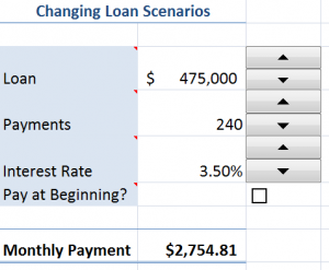
This is the fourth in my continuing series of Excel training video lessons on Adding Form Controls to your worksheets. Here, I demonstrate how to Add Scroll Bar Controls to a Loan Scenario. Form Controls help to make your Excel worksheets “interactive,” and they are great tools to add when you distribute spreadsheets to users who may not be proficient in Excel.

Understand the Cell Link

The key concept to understand with Form Controls is the “Cell Link.” The form controls are merely “drawing shapes” until you actually link them to a cell that controls their output. The “got’cha” step for Scroll Bars – as with Spin Buttons – is that the Maximum Value is 30,000. So, if you want a control to show a loan amount of, for example, $300,000.00 you make the Maximum value 300 and then create a formula that references the “cell link” and multiplies it by 1,000.

In my research on Form Controls, I rarely find authors who mention this point – and, in my experience, this is how most Excel users get “tripped up” when they want to add Form Controls to workbooks to make them interactive. Watch as I walk you through each step in this process.

Please, let me know if this video lesson has helped you to better understand how Excel Form Controls work. Add your comment below – I promise to respond to your comments!

Danny

You can click on this link to view the other videos in my series on Form Controls in Excel.

Learn how to “Master Excel in Minutes – Not Months!”

Learn How to Protect Your Excel Worksheets

Protecting your Excel worksheet is a two-step process. Understand that, by Default, all cells in the worksheet are “locked.”

1) Your first step is to select the input cells that you want your end-user to be able to type in or edit and “unlock” them. That is the “got’cha” step.

2) Next, you go to the Review tab on the Ribbon – in Excel 2007 – and apply the Protection options that you want to be in place for the worksheet.

I like to apply protection to any Excel worksheet that I intend to distribute to end-users. I want them to be able to interact with the data, but I do not want them to be able to change the formulas and formatting that I worked hard to put in place.

Understanding the need to “unlock” input cells while “locking” formula cells is the key to successfully protecting your Excel worksheets. I walk you through two examples in this short video lesson. In addition, I show you how to protect your entire workbook – with or without a password.

This is one of the tips that I include on my DVD, “The 50 Best Tips for Excel 2007.” Click here to purchase it today!

Learn how you can “Master Excel in Minutes – Not Months!”

Create Interactive Excel Forms Using Option Button Controls

This is the third in my series of video lessons that show you how to add Form Controls to an Excel worksheet. Option Buttons, inside a Group Box, are a great way to make your forms “interactive” – to give your end-user multiple options. For example, a choice of shipping methods for their order. Or, to see how different “down payment” options effect their mortgage payments.

The key to understanding how Excel Form Controls operate is to see how the value in the “cell link” changes when you choose an option. The cell link for an Option Button translates a “text expression” into a numeric value. For example, “Surface” translates to “1” for a shipping option.

In this Excel Training Video, I introduce the =CHOOSE() Function. It is rare that I find a client who has ever used this function. Once you see how useful it is, you will start to use it instead of struggling through multiple =IF() Functions. It is really a great “hidden gem” of an Excel Function!

Click on this link to go to my Archive of Excel Video Lessons on Forms. 

You can also find additional groups of related videos by selecting a “Category” from the drop-down menu on the right side bar of any page on my website.

Learn how to “Master Excel in Minutes – Not Months!”

Create User Friendly Excel Forms Using Spin Button Controls

An Excel Form is great way to distribute an Excel worksheet to your customers or field representatives. Most of the time, you do not want them to type values into a cell. You want to make this Form as “user friendly” as possible! You want to add “Spin Buttons” to your form, so that the user can simply click to change cell values up or down in the increments that you want to display.

A perfect example: A Mortgage Loan Scenario where – by clicking the Spin Buttons – your client can see what their monthly payment will be. This is my second lesson covering Excel’s Form Control Tools. Watch as I demonstrate how to “work around” the Form Controls limits of Maximum Amount for a Spin Button (30,000) and also how to increment interest rates by 1/4 of a Percent.

From personal observation, I know that many people start to create an Excel Form and then just give up in frustration. I did too – in the beginning! Watch me demonstrate how to avoid the traps of the “got’cha” steps in this short Excel Training Video.

Check out the great tips that I offer on my DVD, “The 50 Best Tips for Excel 2007.” Click here to start shopping.

Learn how you can “Master Excel in Minutes – Not Months!”

How to Add a Check Box Control to an Excel Form

Judging by the comments that I get from many clients, adding a “Check Box Control” to and Excel Form is not as easy as it appears at first glance.

And, I agree! I, too, struggled with adding Form Controls in Excel. Most of the explanations that I read seemed to add more confusion than clarification!

Spin Buttons in Excel

Spin Button Controls

That is why I created this Excel Training Video: to  lead you through the process; to save you some time and to ease your frustration.

Key Points to Remember:

  1. In Excel 2007, be sure to display the “Developer Tab” on the Ribbon in order to to Insert any Form Control.
  2. Choose the Controls in the “Forms Controls” and NOT in the Active X Controls.
  3. After you “draw” the Control Box on your Form, be sure to select a “Cell Link” to enable the Check Box Control.
  4. Remember that a Check Box Control can only be applied when the result of the Formula or Option is a Logical Value – either a result of  “True or False.”

Don’t be scared off! I find that this is an Excel concept that is better presented “visually.” I struggled for some time when I “read” how to add form controls.

So … I welcome your thoughts – “True or False.” Did I make this easy for you to understand?

Please feel free to add your comments below!

Watch My Video on YouTube

Follow this link to watch my tutorial on my YouTube Channel – DannyRocksExcels

Watch Video Now


Master Excel in Minutes Training Resources

I have created a series of extended length Excel Training Videos. I invite you to visit my secure online shopping site to:

Learn how to “Master Excel in Minutes – Not Months!”

Use an Excel Data Table to See Effect on Multiple Formulas

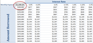
Excel Data Tables are part of the “What-if” Analysis group of tools and commands. In this lesson, I demonstrate how to use a one-input Data Table to show how substituting a series of inputs effects three separate formulas. This is a powerful – and easy – way to get answers to a series of “What-if” questions.

Data Table

2-Input Data Table

Two-Input Data Table

I know that as I learned how to construct Data Tables, it was a lot easier for me to “see” how to set them up rather than to “read about” how they are set up. You can put your series of substitute values in either the “Column running down” or the “row going across” in the data table. To include the three formulas in the Data Table, I simply included “Links” to the formulas in the original assumptions table.

Learn More About “What-if Analysis Tools in Excel

I have identified “What-if” Analysis as one of my “Nine Essential Skills for Excel.” You can learn more about my 4 hour video tutorial package by clicking on either of these links:


Use the Visible Cells Command in Excel to Paste Subtotal Results

Earlier this week a client asked me to help her paste the Subtotal results to a new Excel workbook. She was frustrated and nearly hysterical because her manager needed the results in an hour. If you work with Subtotal reports in Excel I am sure that you share my client’s frustration.

The key to making this work is to use the “Visible Cells Only” command before you copy your selection. You can find this command on the “Find and Select” drop-down menu. If you like keyboard shortcuts, you can use Alt + ; for this command. However, remember to make your selection first!

Watch me demonstrate how this works in this short 4 minute 58 second Excel Video Lesson. You can also view it on iTunes and on my YouTube channel. This is one of the tips that I share on my DVD, “The 50 Best Tips for Excel 2007.”

Learn how you can “Master Excel in Minutes – Not Months!”