My Video Podcast has been downloaded 4,800 times

My iTunes Podcast

Danny on iTunes

OK, so let me brag a little. I launched my Video Podcast, “Danny Rocks Tips and Timesavers,” in June 2010 on iTunes. When I looked at the number of downloads and views, I was amazed to see that the number had surpassed 4,800 – I am thrilled.

Thank you for your support and encouragement. And, one viewer has reviewed my podcast:

Customer Reviews

Concise training      

by ChipAv

These are very specific and concise training modules on individual aspects of Excel and Powerpoint. (Also a few on meeting management and social media.) No nonsense, down-to-business, accurate, and professional. If one of these matches the skill you want to quickly acquire, you should like these.

I invite you to view, download, subscribe or review my video podcasts – either individually or as a whole. Here is the link to my iTunes video podcast:

http://itunes.apple.com/podcast/danny-rocks-excel-tips/id374923275 – If you like what you see, then pass this link on to a friend or colleague.

You can add your comments below and feel free to use one of the Social Media Icons at the bottom of this post.


How to Create a Pivot Table Year-to-Year Comparison Report

One of my viewers asked for my help in creating and Excel Pivot Table Report. She wants to compare the total number of units shipped during three time periods: the years 2008, 2009 and 2010. The trick to producing this report is to drag the field to be summarized – Units Shipped – to the Values Area three times. Then, you change the Value Field Settings to first Sum the Units, then to compare the change in units year-over-year and finally to express this as a percentage of change. This creates a Year-to-Year Comparison Report.

This is a tip that is best demonstrated visually. So, I invite you to watch this 6 minute and 55 second Excel Video Training Lesson.

If you do not have the time to watch the video now, you can use my RSS Feed to deliver it to your computer or you can subscribe to my Video Podcast on iTunes to watch it later.

Learn how to “Quickly Create Pivot Table Reports and Charts”

How to Create and Modify Excel Pivot Tables

How is it possible that the most powerful tool in Excel is also one of the easiest tools to use? An Excel Pivot Table is, in my opinion, the most powerful tool for analyzing data and presenting it as valuable and actionable information. And, an Excel Pivot Table is also one of the easiest tools to use.  

Summarize Data with Pivot Tables

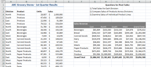
Create a Pivot Table

Create a Pivot Table in six steps:  

  1. With one cell in the data table selected, I clicked on the Insert Tab of the Ribbon and clicked Pivot Table.
  2. I made one change to the default settings – I clicked a cell on the current worksheet to place my Pivot Table.
  3. On the Pivot Table Field List, I placed the Division Field in the Columns area and the Products Field  in the Rows area,
  4. Also on the Pivot Table Field List, I placed the Sales Field in the Values area.
  5. To format the Sales field Subtotals, I Right-clicked a single number and chose Value Field Settings – Number Format.
  6. I also changed the name from “Sum of Sales” to “Sales Revenue.”

It’s that easy! Try it yourself. You will be amazed at how easy it is to create your first Pivot Table. And… as an added bonus, with a Pivot Table you can not harm the underlying data! Pivot Tables work with a “virtual snapshot” of your actual data. Because a Pivot Table uses a “memory cache”  of your data, you can quickly swap your data fields from Rows to Columns to Filters, etc. This is done quickly and efficiently. 

Learn how to “Quickly Create Excel Pivot Table Reports and Charts.”

Here, on the website of The Company Rocks, I offer many free Excel Training Videos to help you get started to create and modify Excel Pivot Tables. Here are the links to the Introductory set of Pivot Table video lessons: 

You can also search for free Excel Pivot Table Video Lessons by following these links: 

“The 50 Best Tips for Excel 2007” DVD

Excel Tip List

Excel DVD Tips

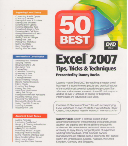
You can also purchase my DVD, “The 50 Best Tips for Excel 2007.”It is affordable and it offers over 5 1/2 hours of focused Excel training tips, tricks and techniques. 

Follow this link to start shopping with my secure shopping cart. I guarantee that you will enjoy my Excel Video Tips. If you are not 100% satisfied, I will refund your purchase price with no questions asked!

List of My Most Popular Posts and Pages

Summer – in the Northern Hemisphere – is now behind us. I went back to survey the videos and pages on my website that had the most views during the Summer of 2010. 

Here is a listing of my “Top 10 Video Posts” and my “Top 5 Pages.” Click on the Links for each title to go directly to the Video Lesson or Page.

The “Top 10 Video Posts” on The Company Rocks Website:

  1. Simplify Data Lookups in Excel
  2. Make Excel Come Alive with Visualization Tools
  3. Build an Accounts Receivable Aging Report
  4. Summarize Multiple Excel Worksheets – Consolidate Data by Position
  5. How to Merge Multiple Excel Workbooks into a Master Budget
  6. Use Pivot Tables to Summarize by Year, Quarter and Month
  7. Perform Break Even Analysis with Excel’s Goal Seek Tool
  8. 2 Reasons to Format Cells Before You Enter Data in Excel
  9. Hide and Show Details in Excel Pivot Tables
  10. Use Vlookup Function to Prepare a Payroll Statement

The “Top 5 Pages” Viewed on The Company Rocks Website:

  1. The Excel Home Page
  2. Index to Excel Video Lesson Topics
  3. List of “The 50 Best Tips for Excel 2007”
  4. Excel Training Videos by Category
  5. The 50 Best Tips for PowerPoint 2007

The Danny Rocks Tips and Timesavers Podcast

During the Summer of 2010, I started my own video podcast at the iTunes Store. These podcasts are free of charge. The video resolution is optimized for viewing on an iPad, iPod or other portable media device.

The DannyRocksExcels Channel on YouTube

Over the past two years I have posted 104 video lessons on my “DannyRocksExcels” Channel on YouTube.

The DannyRocksPowerPoint Channel on YouTube

I maintain a separate channel on YouTube – “DannyRocksPowerPoint”– to post my PowerPoint Tips and Narrated PowerPoint Presentations. I invite you to vist my channel to view, download and share these videos with your friends and colleagues. Click here to go to my YouTube Channel.

“The 50 Best Tips for …” series of DVDs

I offer five DVDs for sale on this website. Click here to start your shopping cart. I guarantee your satisfaction. If you are not 100% satisfied with my DVDs, I will refund your purchase with no questions asked!

You can learn how to “Master Excel in Minutes – Not Months!”

Here is a listing of the DVDs that I offer for sale. Click on the link for each title to go to the list of the tips that I offer on each DVD:

How to Use Excel Lookup Functions to Create a Customer Invoice

Excel has many powerful Lookup Functions. You can use them, for example,  to lookup an Item Number when you know the Product Description. Or to automatically look up the List Price for an Item Number on your customer invoice. In this lesson I show you how to use three Excel Lookup Functions:

  1. The INDEX() Function
  2. The MATCH() Function
  3. The VLOOKUP() Function

I hope that you enjoy learning – and applying – these techniques. I would like to hear from you, so you can either add a comment below or send me an email.

You can receive my new Tips and Timesavers Videos automatically by subscribing to my RSS Feed or to my free podcast on iTunes. Click here to view, download or subscribe to my podcast.

You can purchase any of my 5 DVDs in “The 50 Best Series …” for Excel 2007, PowerPoint 2007, Word 2007, Outlook 2007 and Access 2007 – Click here to open your shopping cart!

Learn how to “Master Excel in Minutes – Not Months!”

How to Share Excel Data with Word Documents

Microsoft Excel is tightly integrated with MS Word. There are several ways to share data that you create in Excel with a Word Document. In this lesson I demonstrate how to copy part of an Excel worksheet and then paste it into a Word document. Here are the techniques that I cover in this short Excel Video Lesson:

  • Paste as a Word Table
  • Paste as a Picture
  • Paste Special as a different type of Picture
  • Paste a Link between the Excel and Word documents – to update the latest sales figures

This is the first in a series of videos where I demonstrate how easy it is to share information between the different programs in the Microsoft Office Suite.

You can see a list of “The 50 Best Tips for Word 2007” by following this link.

You can view and download this video – for free – at the iTunes Store. I invite you to subscribe to my podcast, “Danny Rocks Tips and Timesavers.”

Learn how to “Master Excel in Minutes – Not Months!”

Two Ways to Create a Frequency Distribution in Excel

What is a “Frequency Distribution?” A good example is to see how frequently daily sales are “under $75.00” or how often they range “between $75.00 and $150.00.” Once you know how frequently a result occurs, you can better focus your attention on that particular segment of your business.

In this short 5 minute and 45 second Excel Training Video Lesson, I demonstrate two approaches to creating a Frequency Distribution Report:

  1. Use the =FREQUENCY() Function – this is an ARRAY Function.
  2. In a Pivot Table, Group the Row Labels to produce a Frequency Distribution.

An ARRAY Function has two “Got’cha steps:”

  1. Select all of the cells that will contain the results before your enter your Array Formula.
  2. Use the Ctrl + Shift + Enter keyboard combination to enter your Array Formula.

You can watch this video here on my website, you can download it via an RSS Feed or you can watch it as a Podcast at the iTunes Store.

Learn how to “Master Excel in Minutes – Not Months!”

How to Use an Excel Data Table for “What-if” Analysis

Excel has many tools that give you answers to “What-if” questions. An Excel Data Table allows you to feed a series of “substitute values” into two arguments in a formula. For example, with a Data Table you can:

  • See a table of monthly payments on a loan by substituting both the “Interest Rate” and the “Amount Borrowed” simultaneously.
  • See a table of “Net Payments” by changing both the “Sales Price” and the “Quantity” simultaneously.
  • See the amount that you “tip” a service professional by changing both the “Tip Percentage” and the “Food Total” simultaneously.

As you will see in this Excel Video Lesson, the trick is to understand which series of values are the “Row Inputs” and which series of substitute values are the “Column Inputs.”

Trust me on this: It is easier to “see” how to set up a Data Table than it is to “write a description” of a Data Table. So, I invite you to “see for yourself” how easy it is to set up an Excel Data Table and get answers to two simultaneous “What-if” questions!

Click here to see a Listing of “The 50 Best Tips for Excel 2007.”

Learn how to “Master Excel in Minutes – Not Months!”

When to Use Absolute, Relative & Mixed Cell References in Formulas

In my experience, I find that many Excel users get easily confused when it comes time to use an Absolute or a Mixed Cell Reference in a formula. Let me demonstrate how and when to use the proper cell references, so that you always get the correct result.

Here is what each type of cell reference looks like in a formula:

  • Relative Cell Reference – =A2*B2 when copied down one row becomes = A3*B3
  • Absolute Cell Reference – =A2*$B$2 when copied down one row becomes =A3*$B$2 (Notice the $B$2 Absolute cell reference in the formula)
  • Mixed Cell Reference – =$A2*B$3 when copied down one row becomes = $A3*B$3 and when copied one cell to the right becomes =$A*C$3 (Notice how one part of the cell reference is relative – it moves; and the other part of the reference is Absolute – it remains fixed in place)

Learn how to “Master Excel in Minutes – Not Months!”

Prevent Duplicate Cell Entries with Excel Data Validation

Unfortunately, it is much too easy for a data entry clerk to assign duplicate account numbers. And this is a disaster waiting to happen. To prevent this from happening, use Excel’s Data Validation tool. In this short video lesson, I show you how to use the =COUNTIF() function in the Data Validation dialog box to ensure that only unique account numbers can be assigned to your customers.

I also show you how to extend the range of cells that contain this data validation rule: You use the Paste Special – Validation command.

This is one of “The 50 Best Tips for Excel 2007.” Click here to purchase the DVD using my secure shopping cart.

Learn how to “Master Excel in Minutes – Not Months!”