How to Solve Four Frustrations When Calculating Time in Excel

Have you ever been frustrated when you:

  1. Entered a “Time Value” in a cell only to find that Excel did not recognize it as a “time value?”
  2. Wrote a formula to calculate the elapsed time between “start and finish” only to find that Excel returned a “date” (e.g. 1/15/2008) and not a number?
  3. Wrote a formula to calculate the hours worked for your “Graveyard Shift” (those whose work hours cross Midnight) only to get a cell full of ########?
  4. Used the AutoSum function to calculate the total hours worked in a week only have Excel return a “silly” total like 1.7915?

Well, join the club! Most of my clients have experienced these four frustrations when they try to calculate “time values” in Excel. In this short video lesson, I will demonstrate how to solve each of these four frustrations.

I’d like to receive your feedback on this video lesson. Have you ever encountered this frustation? Did my explanation help you? What additional topics would you like me to cover?

You can email me – danny@thecompanyrocks.com

Here are the steps to follow in this video lesson:

  • Excel stores Time values as decimal numbers. Midnight is 0.00; 6:00 AM is 0.25; Noon is 0.5
  • Be careful when you enter “time values” into a cell. 12:00PM is considered “text.” You need to include a SPACE before the PM e.g. 12:00 PM in order to tell Excel that this is a “time value.”
  • Use this Keyboard Shortcut Ctrl+Shift+~ (Tilde) to see how Excel stores a “time value” in a cell.
  • When calculating “elapsed time”, use a “Custom Format” for  the cell with the Formula E.g. [h]:mm
  • When you calculate “elapsed time” for cells that “cross midnight” you will get ###### as your result unless you use a formula like =MOD((End_Time-Start_Time), 1)
  • When you total “time values” that will exceed 24 hours (E.g. Hours worked in a week) format the cell containing the formula with a “Custom Format” e.g.[h]:mm

Find the Excel Video Lesson that you want – Index to all Excel Topics

News! My DVD, “The 50 Best Tips for Excel 2007” is now availabe to purchase. I invite you to visit my online bookstore for more details.

Trust Your Sources but Verify Your Data’s Accuracy

You may be familiar with the expression, “Trust but Verify!” President Reagan used this phrase when referring to the Soviet Union’s agreement to disarm their missiles. It is also a good approach to follow when you receive Excel data from someone else:

  1. Never open up a data file unless you trust the source.
  2. Never make a decision on the data until you verify the accuracy of the formulas and the structure of the spreadsheet.

In this Excel Video Lesson, I demonstrate how to use the GoTo Special Dialog box to verify the accuracy of your data.

Here are the steps to follow in this lesson:

  1. Choose Edit – GoTo – Special – Formulas to highlight all of the cells containing formulas in the worksheet.
  2. The Keyboard Shortcuts for “GoTo” are Ctrl+G or the F5 Key.
  3. In the “Special” dialog box, you can also choose “Constants.” This may make it easier to spot the cells that are “hard-coded” with a constant value when they should contain a formula.
  4. You can narrow your selection to “Text,” “Logical,” Numeric,” etc. formulas.
  5. Use the Ctrl+~ (Tilde) Shortcut to show the actual formulas in your worksheet.

NEW! Download the Practice File Used in This Excel Training Video

Find the Excel Video Lesson that you want – Index to all Excel Topics

News! My DVD, “The 50 Best Tips for Excel 2007” is now availabe to purchase. I invite you to visit my online bookstore for more details.

Related Videos

The NASCAR Approach to Saving Time in MS Excel

This morning, while I was teaching a class to use MS Excel 2003, a young man in the class called out, “I get it!”

I replied, “That’s great, Ian. What did you get?”

“It’s NASCAR!”

“NASCAR?” I replied – somewhat puzzled.

He explained. “In NASCAR Racing, the pit crews save a second here and a quarter of a second there. That’s how they win the race.”

So, there you go – “It’s NASCAR!” Saving a few seconds here and a few seconds there is how you win the business race. Watch this video to see how to save time when creating multiple formulas.

Here are the steps to follow in this video:

  1. To AutoSum BOTH the Columns AND the Rows with one-click of the mouse:
  2. Select the range of cells containing the values that you want to total PLUS the blank cells immediately to the RIGHT and immediately BELOW.
  3. Click the AutoSum ICON. Amaze your friends.
  4. If you like Keyboard Shortcuts. Instead of clicking the AutoSum Icon, use Alt+=

Find the Excel Video Lesson that you want – Index to all Excel Topics

News! My DVD, “The 50 Best Tips for Excel 2007” is now availabe to purchase. I invite you to visit my online bookstore for more details.

My 5-Star Excel Video Lessons on YouTube

YouTube Logo

YouTube Logo

I have posted several of my MS Excel 2003 Video Lessons on YouTube. The YouTube community votes  or rates individual videos. I’d like to share the results with you. To make it easy for you to view a video that interests you, I have established “Hyperlinks” to take you directly to that video lesson. Simply click on the title and you can view the tutorial.

Here is a listing of my 5-Star Excel Videos on You Tube:

News! My DVD, “The 50 Best Tips for Excel 2007” is now availabe to purchase. I invite you to visit my online bookstore for more details.

The versatile and valuable =IF() Function

MS Excel’s =IF() Function is a very versatile function and it is used in a variety of situations. Watch this short video lesson to learn how to use it when Grading Scores, Calculating Shipping Rates and “Trapping Errors.”

Here are the steps to follow in this lesson:

  1. The =IF() Function requires three arguments: A “Logical Test” – (which will return either a TRUE of a FALSE Response); the Value if “True,” and the Value if “False.”
  2. In my first example I have set up a simple scoring system for grades. For the Value if TRUE, I have entered “Pass.” Notice that the TEXT must be enclosed in ” “.
  3. In my second example, I have “nested” several =IF() functions inside the Value if FALSE Function Argument. You can “nest” up to 7 different IF() Functions in a formula.
  4. Notice how useful the =IF() Function is when you want to “trap an error.” Especially when you are starting to build a spreadsheet and many cells contain Zeros or NULL Values.

Find the Excel Video Lesson that you want – Index to All Excel Topics

News! My DVD, “The 50 Best Tips for Excel 2007” is now availabe to purchase. I invite you to visit my online bookstore for more details.

2 reasons to format cells before you enter data in Excel

Stop! Think! Consider! Develop a plan!

Before you enter any data in your spreadsheets.

Ask yourself questions about your data.  Why?

  1. To save yourself time
  2. To maintain consistency in data entries
  3. To prevent GIGO  (Garbage in equals Garbage out)
50 Best Tips for Excel 2007

Excel Tips

In this video lesson I demonstrate the advantages you will obtain when you:

  1. Stop – before you start to enter data
  2. Pre-plan your data list
  3. Format your data fields / columns BEFORE you make your 1st entry

Here are the steps to follow in this video lesson:

  1. Set up and Format your Column / Field Headers for each data field.
  2. For each Column / Field Header, select the columns and format the cells (Ctrl+1) BEFORE you enter any data.
  3. On the NUMBER tab, choose “Special” to select formats for Social Security #, Phone #, and Zip Code

News! My DVD, “The 50 Best Tips for Excel 2007” is now available to purchase. I invite you to visit my online bookstore for more details.

Find the Free Excel Training Video that you want – Click here to go to my Index of Excel Video Lessons

Excel 2003 Basics – Data Entry

A viewer wrote in to request a few videos that cover “The Basics” in Excel 2003. In this video lesson, I cover the basics of data entry.

Even if you have been using Excel for a number of years, I guarantee that you will pick up one or two tips in this video that will save you time and make you more productive.

Here are the steps to follow in this video lesson:

  1. Excel aligns “text” entries to the left-side of the cell. “Numeric” entries (including Dates & Times) are aligned to the right-side of the cell.
  2. All calculations in Excel MUST start with the =sign. This includes Formulas and Functions. Write formulas that refer to other cells. (Avoid writing formulas that only use constant values.)
  3. When we input data in a cell and press the ENTER key, Excel accepts the entry and makes the cell that is down one row in the column the “Active Cell.”
  4. To input data in the cells of the same row – and continue to use the ENTER key – first select the range of cells in the row.
  5. You can also select a range of cells in adjacent rows and columns. Excel goes down the cells in the column first and then moves automatically to the top row in the next column in your selection.

News! My DVD, “The 50 Best Tips for Excel 2007” is now availabe to purchase. I invite you to visit my online bookstore for more details.

Find the Excel Video Lesson that you want – Index to all Excel Topics

Paste Special Saves You Time – Explore Your Options

I love the Paste Special options in Excel (and Word and PowerPoint.) They save me time. They help to ensure that I am always referring to the latest data. And they help me to be more productive. What’s not to like?

In this video lesson, Danny will demonstrate how to get the most out of each Paste Special option.

Here are the steps to follow in this video lesson:

  1. When you want to copy the “results” of a formula and not the actual formula, choose “Edit, Paste Special, Values.”
  2. If you want to copy the “source formatting” as well as the Values, choose “Edit, Paste Special, Values and Number Formatting.”
  3. To change the orientation (from Vertical to Horizontal, e.g.) choose “Edit, Paste Special, Transpose.”
  4. To ensure that your copied data remains current, choose “Edit, Paste Special, Paste Link.”
  5. You can also use the Paste Special Dialog Box to choose Paste Special “Formats” and “Comments.”
  6. Experiment with Paste Special Add, Multiply, Subtract & Divide.

Find the Excel Training Video that you want – Index to all Excel Topics

News! My DVD, “The 50 Best Tips for Excel 2007” is now availabe to purchase. I invite you to visit my online bookstore for more details.

Related Videos

Create a Calculated Field in Your Pivot Table

When someone wants to see an additional field in your Pivot Table – e.g. to show the “Price per Units Sold,” you create a “Calculated Field.” This is a fairly simple process. In this video, Danny will show you how. This is yet another example of how you can use the power of a Pivot Table to present data the way that you – or your audience – want to see it.

Here are the steps to follow in this lesson:

  1. On the Pivot Table drop-down menu select “Formulas, Calculated Field.”
  2. In the dialog box, write in a Name for your new Calculated Field.
  3. Enter the Formula. Use the Fields in your Pivot Table and any operators (+,-,*,/) Click OK.
  4. Use the Field Settings to change any formatting, etc.

Find the Excel Training Video you want

My DVD, “The 50 Best Tips for Excel 2007” is now availabe to purchase. I invite you to visit my online bookstore for more details.

Get a Free 28 Minute Excel Video Tutorial

Follow this link for information to download – “Introduction to Pivot Tables in Excel 2003”

Use Pivot Tables to Summarize by Year, Quarter and Month

Can you imagine trying to use Excel Subtotals to summarize a long column sales – listed by date? What would you subtotal?  At every change in date?

This would be a nightmare! This would produce a useless report!

Pivot Tables, on the other hand, can provide a summary of dates by month, quarter, and year with just a few mouse clicks!

In this video lesson I show you how to produce that summary. The Pivot Table will transform a long list of data into information that you can use to analyze trends.

Here are the steps to follow in this lesson:

  1. Create a Pivot Table using all of the default settings. Drag the “Date” field into the ROW area and the “Sales” field into the DATA area of the Template.
  2. With 1 cell in the “Date” row selected, choose “Group & Show Detail, Group.” Select Year, Quarter and Month and click OK.
  3. You now have 3 ROWS in your Pivot Table – Year, Quarter & Month. Drag the Year field from the ROW up to the COLUMN area. Hide on of the “Grand Totals.”
  4. Click the Pivot Chart icon to create a Pivot Chart on a new worksheet. Filter the data fields.
  5. Move the Year field back to the Row area. Ungroup the fields to return to the starting point.
  6. To Group by WEEK: Choose “Group & Show Detail, Group” and select DAY. Then select 7 for the number of days in the week.

Find the Excel Training Video that you want – Index of all Excel Topics

Additional Pivot Table Resources

Pivot Table Training Resources

Pivot Table Training Resources

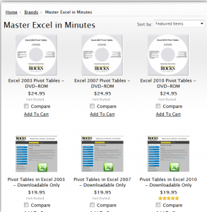
I have published a 90 minute focused video tutorial for Pivot Tables. It is available for each version of Excel -2010, 2007, and 2003. You can purchase it as either a DVD-ROM that I will ship to you or as a Downloadable version that you can work with immediately.

In addition to the 90 minutes of video instruction on Pivot Tables, the package includes:

  • The Excel Practice Files that I used while filming the video tutorial – so that you can practice your new skills using the same files that are on the video.

I invite you to visit my secure online shopping website – http://shop.thecompanyrocks.com – to learn about the many training resources that I offer for sale.

  • A Step-by-step Instructional Guide that you can print out – so that you can use it to take notes as you watch my video tutorial.

Related Video Lessons