How to Use Named Ranges in Existing Excel Formulas

Paste Named Ranges in Formula

Paste Named Ranges in Formula

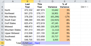
I am a strong proponent for using Named Cell Ranges when creating Excel Formulas. But what if you have already created formulas – formulas that use cell references. How do you insert or apply a newly created named range into an existing Excel Formula?

Simple answer – watch this short video to see me demonstrate how this is done.

Better answer:

Follow These Steps

  1. Activate in-cell formula editing by either double-clicking the formula cell or using the Keyboard Shortcut F2.
  2. Highlight the cell reference that you wish to replace with a named range.
  3. Choose the Name from the “Use in Formulas” drop-down menu. You can also use the F3 Keyboard Shortcut to open the Paste Names Dialog Box.
  4. Repeat these steps to complete replacing additional cell references with named cell ranges.

Learn to Get the Most from Excel

On my DVD-ROM, “The 50 Best Tips for Excel 2007,” I offer 5 1/2 hours of video instruction. You will be amazed at how much more you can get out of Excel when you invest in this valuable resource. I invite you to visit my secure, online shopping website to learn more about the resources that I offer.

Watch Video in High Definition

You can view this Excel Tutorial in High Definition on my YouTube Channel – DannyRocksExcels
Play Tutorial Now

3 Reasons to Create and Use Named Ranges in Excel Formulas

Use Named Ranges in Formulas

Use Named Ranges in Formulas

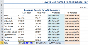
In my opinion, there are three reasons to use Named Range references in Excel Formulas:

  1. They are easier to write. Particularly, if you are referencing cells in another worksheet.
  2. They are easier to remember. Using =Sales – Cost of Goods Sold to determine Gross Profit vs. =A1 – B1
  3. They are easier to explain. Especially, if you are sending an Excel Workbook to a client or a colleague.

Creating Named Ranges in Excel

In this tutorial, I demonstrate two methods for creating a named range:

  1. Select the cells in the range and then type the name in the “Name Box” in the Upper Left Corner of the worksheet.
  2. Select both the cell with the “Name” and the adjacent cells for the range. Then use the Keyboard Shortcut Ctrl + Shit + F3 to open the Create Names from Selection Dialog Box

Remember that all Named Ranges MUST begin with a Letter or an Underscore and they CANNOT contain any Spaces!

Paste Named Ranges into Formulas

If you are using Excel 2007 or Excel 2010, you can take advantage of Formula AutoComplete to quickly and accurately include named ranges in your formulas. In ALL versions of Excel you can use the F3 Keyboard Shortcut to open the Paste Names Dialog Box and select the named range that you wish to paste into your formula.

Additional Resources for Excel

I invite you to visit my secure online shopping website – http://shop.thecompanyrocks.com – where you can preview all of the resources that I offer you.

Watch Tutorial in High Definition

Follow this link to watch my Excel Video in High Definition. My YouTube Channel – DannyRocksExcels – has received over 1 million views!

Watch Video Now

How to Use Excel Formulas and Functions to Analyze Inventory for a Retail Store

Excel Formulas to Analyze Inventory

Excel Formulas to Analyze Inventory

My friend, Alan Friedman, is a CPA and Partner in Friedman Kannenberg and Company, PC. I have been using one of the Excel Worksheets that Alan developed to teach retail store owners and managers how to analyze their inventory. In this lesson, I demonstrate how to write and copy the Excel formulas needed to perform this analysis.

Excel Formulas for Analyzing Inventory

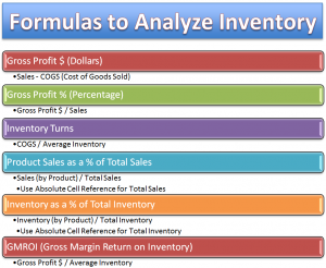
Many retailers use a Point-of-Sale (POS) System that can generate three numbers: Sales by Product Category, Cost of Goods Sold (COGS) by Product Category and Average Inventory by Product Category. Taking these three numbers – also known as “hard-coded” values – you can use Excel Formulas to give you:

  • Gross Profit Dollars (Sales minus COGS)
  • Gross Profit Percentage (Gross Profit Dollars divided by Sales)
  • Inventory Turns (COGS divided by Average Inventory)
  • Product Category Sales as a Percentage of Total Sales (Category Sales divided by Total Sales) – Use an Absolute Cell Reference
  • Inventory by Category as a Percentage of Total Inventory – (Inventory by Category divided by Total Inventory) – Use an Absolute Cell Reference
  • Gross Margin Return on Inventory (GMROI) – (Gross Profit Dollars divided by Average Inventory)

Tips for Entering and Copying Excel Formulas

As I demonstrate in this tutorial, you can write and copy an Excel Formula in one step when you first select the cells to receive the formula and use the Ctrl + Enter Keyboard Shortcut to complete the formula. Instead of clicking on the AutoSum Command or writing =SUM(), use the Alt + = (equal sign) to sum up the values in the adjacent range of cells.

Learn to Improve Your Excel Skills

If you want to learn how to create and use more Excel Formulas and Functions, I have created the Best-selling DVD-ROM, “The 50 Best Tips for Excel 2007.” You can learn more about this resource by visiting my secure online shopping website – http://shop.thecompanyrocks.com

Watch Tutorial in High Definition

I produce my Excel Tutorials in High Definition. Follow this link to view this lesson on my YouTube Channel – DannyRocksExcels
View Tutorial Now

The Basics for Creating and Copying Formulas and Functions in Excel

Relative and Absolute Cell References

Relative and Absolute Cell References

Formulas and Functions are the “core elements” of Excel. It is vital that you have a solid grounding in understanding how formulas and functions work; especially when you need to copy and paste them into other cells.

Relative and Absolute Cell References

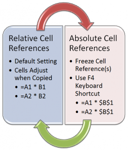
When you use Relative Cell References – the default setting in Excel – the Row numbers and Column letters adjust automatically when you copy and paste a formula.

There are, however, situations where you need to “freeze in place” part of an Excel Formula. For example, you need to “freeze” or use an Absolute Cell Reference to the cell with “Total Sales,” when creating and copying a formula to determine Product Sales as a Percentage of Total Sales.

Copying Excel Formulas

In this tutorial, I demonstrate two methods for copying and pasting formulas and functions:

  • Standard Practice is to select the cell with the formula and use the Ctrl + C Keyboard Shortcut to place the formula cell on the Excel clipboard. Then, after selecting the destination cell(s), use the Ctrl + V Keyboard Shortcut to paste the formula in the new location(s)
  • AutoFill Tool.If you are copying the formula cell into adjacent cells, use the AutoFill tool to do this quickly and accurately!

Tips that You May Not Know

In my experience, many Excel veterans are not familiar with these tips and tricks which I demonstrate in this tutorial:

  • The Ctrl + ~ (tilde) Keyboard Shortcut to “toggle” the Show Formulas view for the active Excel Worksheet.
  • The Alt + Enter Keyboard Shortcut to automatically use the =SUM() Function – for adjacent cells.
  • The F4 Key to automatically add Absolute Cell Reference when creating or editing a formula. For example, converts A1 to $A$1.

Learn More Excel Tips and Tricks

50 Best Tips for Excel 2007

50 Best Tips DVD-ROM

If you enjoy the tips and techniques that I demonstrate in this lesson, then you will really benefit from purchasing my best-selling DVD-ROM, “The 50 Best Tips for Excel 2007.” You can learn more about the resources that I offer by visiting my secure online shopping website – http://shop.thecompanyrocks.com

Watch Tutorial in High Definition

Follow this link to view this Excel tutorial in High Definition on my YouTube Channel – DannyRocksExcels
Play Video Now

How to use Wrap Text and Merge Cells Formatting to Improve Excel Worksheet Appearance

Wrap Text for Labels

Wrap Text for Labels

In this tutorial – the second in my series explaining how a worksheet, that my accountant friend Alan Friedman created, works – I focus on improving the formatting for the column labels and other descriptive text.

Wrap Text for Labels

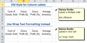
In my experience, I find that many accountants and other financial managers have not mastered the basics of formatting an Excel Worksheet. It seems that they are still using “old fashioned IBM typewriter tricks” when it comes time to create the labels for the columns of data in their spreadsheet.

Case in Point: Using two or more vertical cells to type “Cost of” (Return key on Computer) “Goods Sold.” This “old fashioned” process will lead to multiple problems. For example, improper sorting and filtering of data.

In this tutorial, I demonstrate how to use the Wrap Text command to format a single-cell text label. You will also learn how to use the Keyboard Shortcut Alt + Enter to control where your text “breaks” when wrapping text.

Merge Cells Across Columns

When you have a long, descriptive text – e.g. Your Company Name – it is best to type this into a single cell and then use the Merge Cells Command. Now, when you double-click between Column Letters to automatically expand the width of a column, only the “um-merged” labels in the column are extended in width.

Additional Resources for Tutorial

You can learn “The 50 Best Tips for Excel 2007” on my DVD-ROM. Visit – http://shop.thecompanyrocks.com/50-best-tips-for-excel-2007/ – to learn more about this.

Click on this link to download the Excel Worksheet – created by Alan Friedman – that I use in this lesson.

Watch Tutorial in High Definition

Follow this link to watch this tutorial in High Definition on my YouTube Channel – DannyRocksExcels
View Tutorial Now

How to Apply Alternate Row Shading Using Conditional Formatting in Excel

Alternate Row Shading

Alternate Row Shading w/ Conditional Formatting

This is the first tutorial in a new series. In collaboration with my good friend, Alan Friedman – CPA and partner with the firm Friedman, Kannenberg & Co., PC – I am using Alan’s Financial worksheets to demonstrate how to get the most out of Excel. In this lesson, I show you how to apply Alternate Row Shading – aka “Green Bar Shading” – to a Year-end Inventory Analysis Excel worksheet.

Conditional Formatting in Excel

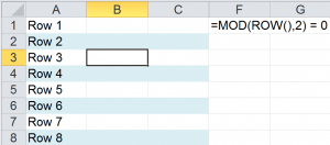
In this lesson, I create a new rule that uses a formula to determine the “condition” – or criteria – that must be met in order to apply the “formatting” to my selection of cells. The “key” to understanding this rule: The formula that you use for this “rule” must return either TRUE or FALSE. The cells – in the selection – that evaluate to TRUE will receive the special formatting – a background shading.

Extending Range of Cells to Receive Conditional Formatting

In general, you can use Excel’s AutoFill Handle to extend Conditional Formatting to adjacent cells. If, however, you want to apply the “Rule Using a Formula” to non-adjacent cells, first copy a cell that contains the Conditional Formatting. Then, use Paste Special – Formatting to apply this rule to your new selection of cells.

Resources for This Tutorial

I invite you to visit my secure online shopping website – http://shop.thecompanyrocks.com – to preview all of the resources that I offer to you.

Please visit the Friedman, Kanneberg & Co. website to download the worksheet used in this series of lessons – and other seminar handouts.


Watch Tutorial in High Definition

Follow this link to watch this Excel Tutorial in High Definition on my YouTube Channel – DannyRocksExcels

Play Video Now

How to Create Custom Views of a Worksheet in Excel

Custom Views in Excel

Custom Excel Views

This is Part 2 in my series of video tutorials demonstrating the Commands found on the View Tab of the Excel Ribbon. Building on the concepts that I demonstrated in Part 1 (“How to Freeze Row and Column Labels While Scrolling in Excel”), I now show you how to save these settings as a Custom View.

Create a Custom View in Excel

  1. Display the settings that you wish to save as a Custom View – e.g. Changing the ZOOM Level of Magnification, Freezing Rows or Columns, etc.
  2. From the View Tab on the Ribbon, choose the Custom Views Command.
  3. In Custom Views Dialog Box, click Add; Give your View a Name and Click OK.
  4. Remember to Save your Excel Workbook. To test your custom view, I recommend that you revert to your normal or default view and save that version. Then close the workbook and reopen it. Now, it will display the last view displayed when you saved the workbook. Click on the Custom Views Command and select the Custom View that you recently added; the Custom Settings will now display.
  5. Add – and Save – additional Custom Views.

Custom Views are Worksheet Level Views

When you create a Custom View, it only applies to the Excel Worksheet where you created it. In fact, while you “Show” a Custom View, all other Worksheets in the Active Workbook are NOT available.

Excel Tables and Custom Views

 There is one “gotcha” with Custom Views. If you have formatted a data set as an Excel Table on ANY worksheet in the workbook, ALL Custom Views are blocked out. Watch  this video to see how to “work around” this roadblock.

Online Shopping at The Company Rocks

I invite you to visit my secure online shopping website – http://shop.thecompanyrocks.com – to preview all of the resources that I offer you.

Watch Tutorial in High Definition

Follow this link to view this Excel Tutorial in High Definition on my YouTube Channel – DannyRocksExcels
Play Video Now


How to Freeze Row and Column Labels While Scrolling an Excel Worksheet

Split Panes on Worksheet

Split Panes on Worksheet

This is Part 1 in a multiple part series of tutorials. I am responding to the requests of several viewers who want to know the best ways to view an Excel Worksheet.

Freeze Panes and Split Bars

In this tutorial, I demonstrate how to use the three commands on the Freeze Pane Menu:

  1. Freeze Top Row
  2. Freeze Panes – Rows above and Columns to the left of the Active Cell
  3. Freeze First Column

When you need more flexibility to control the visible panes on your worksheet, use the Split Bars. I show you how to apply, modify and remove Split Bars – Vertical and Horizontal – on your worksheet.

With the Split Bars, you gain additional Navigation Scroll Bars – One above the Split and one below the Split with a Horizontal Split Bar. And, one to the left and one to the right of the Vertical Split Bar.

Go to Additional Tutorials in this Series

Visit My Online Shopping Website

I invite you to visit my secure online shopping site – http://shop.thecompanyrocks.com – to preview all of the resources that I offer you.

Watch Tutorial in High Definition

Follow this link to watch this Excel Tutorial in High Definition on my YouTube Channel – DannyRocksExcels
Watch Video Now

Click below to start watching this tutorial now.


How to Clear All Underlying Cell Formatting in Excel

Clear Underlying Formatting

Clear Underlying Formatting

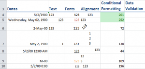
Have you ever typed data or a formula in a cell only to be surprised by the result? For example, you type in a number and then, unexpectedly,  Excel displays a Date or a Time in that cell. This happens frequently when you reuse an older Excel Worksheet of if you start working on a worksheet that a colleague or client has sent you.

Why does this happen?

Clear All Underlying Cell Formatting

In my experience, I have found that many Excel users mistakenly think that pressing the DELETE Key will “erase” the cells in the selection. No, No, No. The Delete key only erased the cell content – the data, text or formulas entered or pasted into the cell(s). The Delete key does NOT remove the Underlying Cell Formatting!

In this tutorial, I demonstrate how to remove the underlying cell formatting while leaving the cell Contents in place.

Topics Covered in this Tutorial

  • Using the Clear Formatting Command
  • Adding the Clear Command to your Quick Access Toolbar
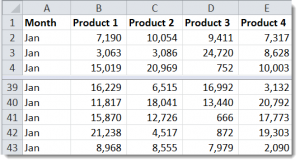
  • Using Go To Special to Find and Select all cell that use either Conditional Formatting or Data Validation
  • Finding the Last Cell in your worksheet – you may be surprised to find a “remote cell” is NOT Blank!

View All the Resources that I Offer

I invite you to visit my secure online shopping website – http://shop.thecompanyrocks.com – to preview all of the resources that I offer.

Watch this Tutorial in High Definition

Follow this link to view this Excel Tutorial in High Definition on my YouTube Channel – DannyRocksExcels


Summarizing Employee Hours Worked and Vacation Time over 52 Weeks in Excel

Sum Across Worksheets

Sum Across Worksheets

This is the third episode in my series of Excel Tutorials where I share my best practices for creating an Excel Workbook that contains 52 weeks of Employee Time Cards. In this lesson, I focus on techniques to Summarize – or Consolidate – the hours worked or taken as vacation, by each employee, over a period of several weeks.

Sum Across Worksheets

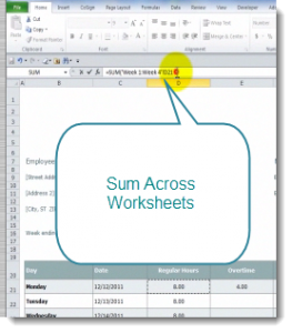
This is a great tip to learn! In my experience, I find that very few experienced users of Excel know that you can do this! This will eliminate the hassle of linking to a cell in individual worksheets to create your formula. There is, after all, a limit to the number of characters that you are allowed in a formula!

Consolidate Data By Position

Since each worksheet in this workbook is identical in structure, Data Consolidation is simple. Provided, that is, that you remember to “Add” each worksheet range reference in the Dialog Box. In this example, I have “created a link” to each worksheet so that the data can be easily updated.

Links to Other Tutorials in this Series

Shop for Additional Resources

I invite you to visit my new, secure online shopping website – http://shop.thecompanyrocks.com – where you can preview all of the resources that I offer you.

Watch Tutorial in High Definition

Follow this link to view this Excel Tutorial in High Definition on my YouTube Channel – DannyRocksExcels