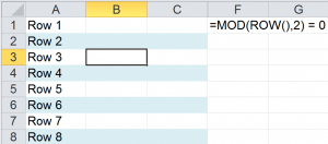
This is the first tutorial in a new series. In collaboration with my good friend, Alan Friedman – CPA and partner with the firm Friedman, Kannenberg & Co., PC – I am using Alan’s Financial worksheets to demonstrate how to get the most out of Excel. In this lesson, I show you how to apply Alternate Row Shading – aka “Green Bar Shading” – to a Year-end Inventory Analysis Excel worksheet.
Conditional Formatting in Excel
In this lesson, I create a new rule that uses a formula to determine the “condition” – or criteria – that must be met in order to apply the “formatting” to my selection of cells. The “key” to understanding this rule: The formula that you use for this “rule” must return either TRUE or FALSE. The cells – in the selection – that evaluate to TRUE will receive the special formatting – a background shading.
Extending Range of Cells to Receive Conditional Formatting
In general, you can use Excel’s AutoFill Handle to extend Conditional Formatting to adjacent cells. If, however, you want to apply the “Rule Using a Formula” to non-adjacent cells, first copy a cell that contains the Conditional Formatting. Then, use Paste Special – Formatting to apply this rule to your new selection of cells.
Resources for This Tutorial
I invite you to visit my secure online shopping website – http://shop.thecompanyrocks.com – to preview all of the resources that I offer to you.
Please visit the Friedman, Kanneberg & Co. website to download the worksheet used in this series of lessons – and other seminar handouts.
Watch Tutorial in High Definition
Follow this link to watch this Excel Tutorial in High Definition on my YouTube Channel – DannyRocksExcels

