My New DVD – The 50 Best Tips for MS Excel 2007 is now on sale

50 Best Tips fo MS Excel

New! Now available from the online store at www.thecompanyrocks.com

Do you ever have one of those “A-ha” moments? You know – those moments when everything falls into place. When everything becomes crystal clear. When you finally “get it!”

Well, here is your opportunity to experience 50  “A-ha” moments. Here is a great way for you to learn “The 50 Best TIps, Tricks, and Techniques for Microsoft Excel 2007.”

I spent almost three months filming these short Excel training videos. I worked hard to create this DVD in order to make it easy for you to learn how to remain productive at work while learning to use the new Excel 2007 interface.

And, the Excel 2007 interface is really quite different.

So different, that many long-time Excel users just give up on it and return to the tried and true Excel 2003 program.

And that is too bad. Because, Excel 2007 allows you to perform so many business tasks faster and better. But … first, you must get over “the initial learning curve” to understand how to navigate in Excel 2007.

This DVD makes it easy for you to learn how to use Microsoft Excel 2007 – guaranteed!

In selecting the 50 Best Tips for Excel 2007, I wanted to include tricks that all Excel users could put to use – now! I include tips at the Introductory, Intermediate and Advanced levels.

Each lesson is short – five to six minutes on average – and focused on just one topic. Each lesson on the DVD is self-contained – I teach you how to solve one problem per lesson.Overall, the DVD contains 5 1/2 hours of training on Excel 2007!

This DVD is available exclusively from the SkillPath Seminars bookstore. They are offering it for sale at the introductory price of $49.95 Here is a link to the demonstration / order now page.

I am proud of this product. I know that you will gain some new insights into how to get the most out of Excel 2007. I welcome  your feedback. Please drop me a note  – danny@thecompanyrocks.com Or … add your comments below for all readers to share.

Thank you for your support!

Danny Rocks

Be Careful with Calculated Items in Pivot Tables

Let me warn you – Calculated Items in Pivot Tables can produce incorrect results! Calculated Items can be useful – in special circumstances. However, don’t use a Calculated Item to create a Quarterly Summary. It is too easy to accidentally “double” your sales! And, this will not earn you any special bonus. In fact, it may harm your reputation as an Excel expert. So be very careful before you create a Calculated Item.

Review my Excel Training Video on Grouping Data to see the preferred way to produce a Quarterly Summary in a Pivot Table.

Here are the steps to follow in this lesson:

  1. You use a Formula to Calculate an Item from the values on one of the Fields in your Pivot Table.
  2. Select one value in the Field where you want to create the Calculated Field.
  3. In this lesson, I selected a Month and then from the Drop-Down Menu on the Toolbar I chose Formula – Calculated Item,
  4. I named the Calculated Item Q1 (1st Quarter) and for the Formula I clicked = January+February+March. Click Add and then click OK.
  5. As you can see, the new Q1 Item actually “doubled” the existing sales for January – March. That is not what you were looking for!
  6. To remove the Calculated Item, select it and then from the drop-down select Formulas – Calculated Item. Highlight Q1 and click Delete – OK.
  7. Review my video to see how to Group Data to produce the Quarterly Summary in the Pivot Table.

Search My Index of Excel Training Videos to find the topic you want to view

DVDs of The 50 Best Tips for Excel and PowerPointNew! Danny’s DVD Training Series, “The 50 Best Tips for …” is now available at the online store for The Company Rocks

Group Data in Pivot Table for Quarterly Report

During a recent Excel training class, one student asked me if was possible to create a Quarterly Summary Report in a Pivot Table. Yes, it is quite easy to do this – as you will see in the video.

In the Data Set that we are using for this Pivot Table we have four territories and 12 months of sales for each territory over a one year period. The Months (Jan, Feb, etc.) are not actual dates (e.g.1/1/08,) they are Labels.

In an earlier video, I showed you how easy it is to create new fields for Months, Quarters & Years from a Date field. Because our months are Labels, we will GROUP the Months to create the 1st, 2nd, 3rd, and 4th Quarters in our Pivot Table.

Here are the steps to follow in this lesson:

  1. Create a Pivot Table using the default settings in the Pivot Table Wizard. Place the Months in the Row area, the territory in the Column area, and the Sales in the Data area.
  2. Select the Labels January, February, March. On the Pivot Table drop-down menu select Group & Show Detail – Group.
  3. Rename the generic label (Group1) to 1st Qtr.
  4. Follow the same sequence of steps to create Groups for the 2nd, 3rd, and 4th Quarters.
  5. Rename the new, generic field (Month2) Quarter.
  6. Use the Toolbar Commands to Hide & Show Detail as desired.

NEW! Download the Excel Practice file that I used in this video

Search the Index of Excel Lessons to find my training video listed by topic

New! Danny’s DVD Training Series, “The 50 Best Tips …” is now available at the online store for The Company Rocks

Related Videos

Change Pivot Table Grouping to a Fiscal Quarter

While I was training a class to use Pivot Tables this week, I showed them how to Group Dates by Month, Year & Quarter. They liked that a lot – it’s a great feature! However, one student said, “My company is on a Fiscal Year. Is it possible to change the grouping of the Quarters from a Calendar Year to a Fiscal Year?”

Yes! There are several ways to do so. In this Excel Video Lesson I demonstrate the easiest way.

Here are the steps to follow in this Excel Training Video:

  1. Create the Pivot Table. In this example we drag the “Date Field” to the “Row Area” and drop the “Sales Field” into the “Data Area.”
  2. Select one cell in the Date field and from the Pivot Table drop=down menu choose Group & Show Detail – Group. Highlight Month & Quarter. Click OK.
  3. We now have a new “Outer Row” filed – Quarter – in our Pivot Table. However, the grouping reflects a Calendar Year. We need to change this to a Fiscal Year.
  4. Select each label, in turn, and edit the name in the Formula Bar.
  5. To change the Order of the Quarters: Right-click the 4th Quarter label and choose Order – Move to End.
  6. Edit the Field Settings for the Quarters Field. Add in the SUM Subtotal.
  7. Make the Quarterly Subtotals & Grand Total rows Bold.
  8. Double-click any Quarterly Label to Hide the Details. Use the Icons on the Toolbar to Show / Hide details for each group to suit your needs.

Looking for a specific Excel Video Lesson? Click here for an Index of all Excel Training Topics

Do you want to see a list of all of my Excel Pivot Table Video Lessons? Click here to go to my Pivot Table Archive.

News! My DVD, “The 50 Best Tips for Excel 2007” is now available to purchase. I invite you to visit my online bookstore for more details.

Top Excel Posts in September 2008

Here is a classified listing of the most popular postings and Video lesson blog entries on my site during the month of September, 2008:

Information about The Company Rocks Excels

Filtering Excel Data

Time-Savers in Excel

Pivot Tables in Excel 2003

50 Best Tips for Excel 2007

Excel Tips

News! My DVD, “The 50 Best Tips for Excel 2007” is now availabe to purchase. I invite you to visit my online bookstore for more details.

Use Pivot Tables to Summarize by Year, Quarter and Month

Can you imagine trying to use Excel Subtotals to summarize a long column sales – listed by date? What would you subtotal?  At every change in date?

This would be a nightmare! This would produce a useless report!

Pivot Tables, on the other hand, can provide a summary of dates by month, quarter, and year with just a few mouse clicks!

In this video lesson I show you how to produce that summary. The Pivot Table will transform a long list of data into information that you can use to analyze trends.

Here are the steps to follow in this lesson:

  1. Create a Pivot Table using all of the default settings. Drag the “Date” field into the ROW area and the “Sales” field into the DATA area of the Template.
  2. With 1 cell in the “Date” row selected, choose “Group & Show Detail, Group.” Select Year, Quarter and Month and click OK.
  3. You now have 3 ROWS in your Pivot Table – Year, Quarter & Month. Drag the Year field from the ROW up to the COLUMN area. Hide on of the “Grand Totals.”
  4. Click the Pivot Chart icon to create a Pivot Chart on a new worksheet. Filter the data fields.
  5. Move the Year field back to the Row area. Ungroup the fields to return to the starting point.
  6. To Group by WEEK: Choose “Group & Show Detail, Group” and select DAY. Then select 7 for the number of days in the week.

Find the Excel Training Video that you want – Index of all Excel Topics

Additional Pivot Table Resources

Pivot Table Training Resources

Pivot Table Training Resources

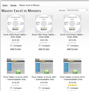
I have published a 90 minute focused video tutorial for Pivot Tables. It is available for each version of Excel -2010, 2007, and 2003. You can purchase it as either a DVD-ROM that I will ship to you or as a Downloadable version that you can work with immediately.

In addition to the 90 minutes of video instruction on Pivot Tables, the package includes:

  • The Excel Practice Files that I used while filming the video tutorial – so that you can practice your new skills using the same files that are on the video.

I invite you to visit my secure online shopping website – http://shop.thecompanyrocks.com – to learn about the many training resources that I offer for sale.

  • A Step-by-step Instructional Guide that you can print out – so that you can use it to take notes as you watch my video tutorial.

Related Video Lessons