Create an Accounts Payable Summary Report in Excel

Accounts Payable Status Summary

Accounts Payable

Here is another video lesson that I created to answer a question from one of my viewers. In this case, the request is for help in creating an Accounts Payable Summary Report in Excel.

Formula to Create Label for Status

My viewer wants to know how to create one formula that will report the status of an Invoice as “Paid,” “Pay Now,” or “Delay.” To do this I “nested” one IF() formula inside another IF() formula. I used the ISBLANK() function as my first “logical test” in the formula. ISBLANK returns either TRUE or FALSE, so it is a good Function to become familiar with.

One of my “best practices” when learning how to “nest” IF Formulas, is to create each one separately – to test the results – and then copy and paste them into the combined formula.

Use SUMIF() Function to Total Status

Now, that your formula returns a status label for each invoice, you can use the SUMIF Function to search in the Named Range “Status” for the cells that match the criteria (Paid, Pay Now, Delay) and then Sum the Invoice Amounts for each category.

Watch This Video in High Definition on YouTube

Here is the link to my YouTube Channel, DannyRocksExcels, where you can watch this in High Definition.

Download this Excel Workbook

Follow this link to go to my Public SkyDrive to download this workbook to practice with.

How to Search For and Use Text Strings in Excel

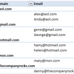
A viewer asked for my help in creating a report that will group his customers’ email addresses by their “domain name.” For example, he wants to be group all customers with gmail addresses . Likewise, his  customers’ yahoo mail, aol.com accounts, etc.

Pivot Table for Email Domains

Pivot Table Email Domains

I immediately decided to use two powerful Excel tools to produce this report:

  1. Text-to-Columns to create two columns (name and domain) from one text value (the email address).
  2. Pivot Table Report to group and present customer emails by domain name.

Both tools work great and I produced the report with only a few mouse clicks!

The response that I got from my viewer was, “That’s great Danny. But …”

It turns out that the viewer wanted to have the Domain Names as the Field Headers and to show each customer’s email address as a row going down vertically in the corresponding field. To give my viewer the report that he wanted, I used these tools and techniques:

  • I returned to the Pivot Table to copy the unique list of domain names.
  • I used Paste Special – Transpose to convert the vertical list of domain names into a horizontal row of Field Headers.
  • I began to build my “Mega-formula” by taking “baby steps” – i.e. I created one formula and then “nested” it inside additional formulas and functions.
  • For the first “baby step” formula I used the SEARCH() Function.
  • Next, I “nested” this formula as the “logical test” inside an IF() Function.
  • In order to “hide” all of the formula error signs, I nested both of these functions inside the NEW IFERROR() Function.
  • IFERROR() was introduced in Excel 2007 and I now consider it to be “indispensable!” This function, alone, makes upgrading to either Excel 2007 or Excel 2010 a “nobrainer” decision!

I enjoy answering questions from my viewers. Many of these questions can be answered from one of the lessons on my DVD-ROM, “The 50 Best Tips for Excel 2007.” For the rest, I try to create a video lesson that demonstrates how to get the answers that you – my viewers and customers – are looking for.

Keep your questions and suggestions coming! I enjoy receiving feedback from you!

I invite you to subscribe to my RSS Feed on Feedburner to be automatically notified whenever I publish a new Excel Video Tutorial.

Watch this Excel Video in High Definition on YouTube

Here is the link to watch this video on my YouTube Channel – DannyRocksExcels

Learn the powerful SUMIF Function

Here are the steps to follow in this lesson:

  1. Type =sumif( and then click the FUNCTION WIZARD to enter the ARGUMENTS.
  2. Enter the range of data that you wish to SUM as the 1st Argument.
  3. Identify the Criteria to evaluate e.g. “>500″ – (enclose the Argument inside ” “) as the 2nd Argument.
  4. The 3rd Argument is OPTIONAL. You can leave this empty if you want to SUM the same range of data from your 1st Argument.

NEW! Download the Practice File from this Lesson:

Find the video lesson that you want – Index to all Excel Topics

News! My DVD, “The 50 Best Tips for Excel 2007” is now available to purchase. I invite you to visit my online bookstore for more details.

Related Videos