Get My New Popular Keyboard Shortcuts for Excel Chart – It’s Free When You Register

Click the link below to download my chart of Excel Keyboard Shortcuts as a PDF:
Excel Keyboard Shortcuts

Preview Excel Keyboard Shortcuts

 Hello and Welcome – to my new “Members Only” section of The Company Rocks website! 

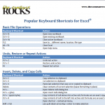
I just published a new five-page Chart – “Popular Keyboard Shortcuts for Excel.” It is free for you to download as a PDF. 

This, along with additional content, will soon be inlcuded in my new “Exclusive Membership Content” area on my website. 

My Exclusive Membership Site is not quite ready to launch. So, I am offering this chart for you to download as a PDF from this post. 

To get this chart, click on this link –  

CR – Updated Chart of Popular Excel Keyboard Shortcuts 

New! Download My Free 50 Minute Video Recording Demonstrating Excel Keyboard Shortcuts

Click this link to learn how you can download my new “extended length” video recording. It is “free of charge!”

I am proud of the way my Excel Keyboard Shortcuts Chart turned out – and I think that you will get a lot of value out of this free resource. I organized the Keyboard Shortcuts by the following Tasks:

Excel Keyboard Shortcuts

  • Basic File Operations
  • Undo, Restore or Repeat Actions
  • Insert, Delete, and Copy Cells
  • Edit Data
  • Show / Hide Columns and Rows
  • Select Contiguous Cells
  • Navigate Within a Worksheet
  • Navigate Between Workbooks
  • Find, Replace, and Go To
  • Enter Data
  • Work with Cell Comments
  • Work with Names for Cells and Ranges
  • Work with Formulas and Functions
  • Work with Formula Precedent and Dependent Cells
  • Print Worksheet
  • Formatting Cells and Text
  • Work with Subtotals and Outlines
  • Work with Tables, Lists, and Filters
  • Work with Charts
  • Work with Excel Windows and Open Applications

So, as you can see, this is a comprehensive – but not exhaustive – list of the best Keyboard Shortcuts for Excel. I took care to ensure that these Keyboard Shortcuts will work for all versions of Excel from 2003 through version 2010. 

The 50 Best Tips

The 50 Best Tips Series

I have several video lessons that cover keyboard shortcuts on my DVD-ROM, “The 50 Best Tips for Excel 2007.” It is a best-seller and it is now on sale! Use Coupon SAVE-20-PCT at checkout and save 20% on any puchase at my online store. Click here to open a secure shopping cart

And let me know your thoughts on my Excel Keyboard Shortcut Chart. Do you have a favorite Keyboard Shortcut that you want to share with our readers? Add your comments below.

Learn how to “Master Excel in Minutes – Not Months!”
How to Add a Combo Box Control to an Invoice in Excel

If you are creating or modifying an Invoice Form in Excel, you will want to add a Combo Box Control to allow users to select products from a listing. The key in formatting your Combo Box Control is to choose the correct cell to contain the “Cell Link.”

Cell Link in Form Control

I think that you will benefit from “seeing how this is done” in this video lesson. I know that I always struggled with “reading about” Excel Form Controls. Once you see how important the “Cell Link” placement is, you will better understand how Combo Box Controls work.

Use INDEX Function

Once we have formatted the Combo Box, we need to be able to look up other values to place on our Invoice. In this example I demonstrate how to use the INDEX() Function to lookup the “Unit Price” for each product selected from the Combo Box list on the Invoice. As a best practice, I recommend that you use “Named Ranges” for the “array” that you Index. The INDEX() Function has three arguments:

  1. The ARRAY to Index – In this case our “named range” with three fields (Product Name, Unit Price, Cell Link)
  2. The ROW reference – In this case the cell in the ARRAY that contains our CELL LINK for the Combo Box
  3. Optionally, the COLUMN reference – in this case “2” for the 2nd Column in the ARRAY (Unit Price)

Let me know if my videos in this series have helped you to understand how to use Form Controls in Excel. It took me some time to figure out how they worked; I hope that I can save you some time and ease your frustration in apply them to your forms. Add your comments below or send me an email – danny@thecompanyrocks.com

Find Additional Videos for Form Controls in Excel

Form Controls include Option Buttons, Spinners, List Boxes and more. Here is a link to the other videos in my series on Form Controls in Excel.

Watch Tutorial on YouTube

If you prefer, follow this link so that you can watch this video on my YouTube Channel – DannyRocksExcels

Resources Available at My Online Shopping Site

I invite you to visit my new, secure online shopping site  where you can Learn how you to “Master Excel in Minutes – Not Months!

How to Use Excel Lookup Functions to Create a Customer Invoice

Excel has many powerful Lookup Functions. You can use them, for example,  to lookup an Item Number when you know the Product Description. Or to automatically look up the List Price for an Item Number on your customer invoice. In this lesson I show you how to use three Excel Lookup Functions:

  1. The INDEX() Function
  2. The MATCH() Function
  3. The VLOOKUP() Function

I hope that you enjoy learning – and applying – these techniques. I would like to hear from you, so you can either add a comment below or send me an email.

You can receive my new Tips and Timesavers Videos automatically by subscribing to my RSS Feed or to my free podcast on iTunes. Click here to view, download or subscribe to my podcast.

You can purchase any of my 5 DVDs in “The 50 Best Series …” for Excel 2007, PowerPoint 2007, Word 2007, Outlook 2007 and Access 2007 – Click here to open your shopping cart!

Learn how to “Master Excel in Minutes – Not Months!”

Two Ways to Produce an Executive Summary of an Excel List

On one of the technology blogs that I follow, there is a debate over the best way to produce an Executive Summary of the information in an Excel Data List. Some people like the idea of using Excel’s =SUMIF() Function for this while others recommend creating a Pivot Table as the summary.

You decide – after watching this short video demonstration using both approaches. And, add a comment or drop me an email to let me know your thoughts.

This Excel Video Lesson is available for you to download as a Podcast on iTunes.

Follow this link to go to the “Danny Rocks Tips and Timesavers” podcast.

Learn how to “Master Excel in Minutes – Not Months!”

How to Create Scenarios in Excel

Scenarios are part of Excel’s “What-If” Analysis tool set – aka Data Analysis. Use Scenarios when you need to know what the result will be when you change one or more variables in one or more  situations (scenarios).

Frequently, I create Scenarios to define  a “Good, Better, Best” or “Worst Case, Best Case, Case Most Likely” outcome.

In this short Excel Training Video, I demonstrate how to create, edit,  and report four Scenarios for a Monthly Office Expense Budget.

These are the steps used in this Excel Video Lesson:

  • Create (or open) an Excel worksheet that contains a formula. Identify the formula and the precedent  cells that feed into the formula.
  • Select the “target cell” – the cell that contains the formula whose result will change with each Scenario.
  • Choose TOOLS – SCENARIOS and follow the directions in the Create Scenario dialog box.
  • First, click ADD. Name the Scenario. Click OK. Confirm that you have selected the “Target Cell” and then click / type in the “Changing cells.” The Changing cells should be either direct or indirect precedents to the Target cell formula. Click Add. Add additional Scenarios as desired.
  • Click on the name of your Scenario and select SHOW to display the changing cell values and the new result in your target cell.
  • If you wish, choose SUMMARY to create a summary report in a separate worksheet.
  • I strongly recommend that you create named cells and use them in the formulas and changing cells of your Scenario.

NEW! Download the Excel Practice file used in this lesson:

Use my Index to search for the free Excel Training Video that you want to view.

New! Danny’s DVD Training Series, “The 50 Best Tips …” is now available at the online store for The Company Rocks

Related Videos

Simplify Data Lookups in Excel

In this Excel Video Lesson I demonstrate a great tip that dramatically simplifies data lookups!

Yes, learning how to use the Lookup Functions (VLOOKUP, HLOOKUP, MATCH, INDEX) is important. But, there is an easier way to answer some simple questions about you data.

In this video, I show you how to use the combination of “Named Ranges” and the “Intersection Operator” – the SPACE – to return the value at the intersection of a specific column and specific row. This “tip” is guaranteed to save you time and simplify your data lookups!

Here are the steps to follow in this lesson:

  1. Create “Named Ranges” for your data set.
  2. Use the “Intersection Operator” – the SPACE – in your formula. e.g. =Region_2 Week_16
  3. It’s that simple!

NEW! Download the Excel file that I used in this video lesson:

simplify-data-lookups

Looking for the answer to your Excel Questions? Use my Index of Excel Topics to find the right video

News! My DVD, “The 50 Best Tips for Excel 2007” is now available to purchase. I invite you to visit my online bookstore for more details.

Related Video Lessons

I Have 21 Excel Videos Rated 5-Stars on YouTube

YouTube Logo

YouTube Logo

Here is a listing of my 21 Excel Video Lessons that are rated “5-Stars” on YouTube.

I hvae organized the videos by category. The First Hyperlink will take you to to the videos on this site. The “indented” Hyperlink will take you to the videos on my YouTube site –  DannyRocksExcels.

I hope that you find a few tips to save you time or answer a question. I welcome your feedback. Enjoy!

Pivot Tables

“What-if” Analysis

Consolidation and SubTotals

Filter & Sort Lists in Excel

Financial Functions in Excel

Logical & Lookup Functions in Excel

Text Functions

Formula Auditing

Formatting and Conditional Formatting

Paste Special Options

Excel Charts

News! My DVD, “The 50 Best Tips for Excel 2007” is now available to purchase. I invite you to visit my online bookstore for more details.

Related Videos

Use the =SUMIF() Function to Tally YTD Sales

Many of my clients keep a “running total” of sales. They put “Dates” in Column “A” and enter each day’s sales in Column “B.” Next is Column “C” which contains the formula =SUM(B$:B250). That is fine – it works.

However, if you use the =SUMIF() function to total Year-to-Date (YTD) Sales you gain flexibility, save space and save time – because you do not have to scroll down several screens to see your YTD Sales total!

In this video, I show you how to use “Named Ranges” in a =SUMIF() Formula to keep track of your cumulative sales total.

Here are the steps to follow in this lesson:

  1. Traditionally, you use a formula like =SUM(B$3:B250) to give you a “running total” for YTD Sales.
  2. The=SUMIF() Function returns the SUM of vales that meet a “Single Criterion” (the IF portion) .
  3. The 1st Argument is – What is the Range that you want your criteria to evaluate? Consider “Naming” this Range – it makes it easier to write your formula and explain your formula.
  4. The 2nd Argument is – What is your criteria? Be sure to use this syntax – “Comparison Operator”
  5. In the video example we also need to include the “&” to join the cell “D2.” Cell “D2,” in this example, contains the Function =TODAY()
  6. The 3rd Argument is – What Range do you want to SUM to return the values that meet your Criteria?
  7. The =DATE() Function returns the serial number for a specific date. It requires 3 Arguments. =Date, Year, Month, Day)
  8. You will save time and gain productivity when you “Name Cells and Ranges” and then you them in your formulas.
  9. Use the F3 shortcut key to “Paste Names” into your formulas.

News! My DVD, “The 50 Best Tips for Excel 2007” is now available to purchase. I invite you to visit my online bookstore for more details.

Find the Excel Video Lesson that you want – Index to all Excel Topics

3 reasons to use named cells and ranges in Excel forumlas

I use named cells, ranges and constants in my Excel formulas and workbooks for 3 reasons:

  1. They are easier to explain (to others and to myself 6 months after I create a formula.)
  2. They are easier to adapt (to other locations in the workbook – absolute cell references not required!)
  3. They are easier to update (especially named constants in formulas when e.g. rates change.)

These are the steps to follow in this Excel training video:

  1. Select the cells that you want to name and also the labels in the left column and top row.
  2. Choose, Insert, Name, Create. Make sure that Left column and top row are selected.
  3. To verify that your names have been created, click the Name box drop down list of names. Select a name and Excel takes you directly to that cell or range.
  4. To substitute Name cells and ranges in existing formulas: Choose Insert, Name, Apply, OK
  5. When you are writing a new formulas and you want to use a name, use the F3 “Paste Name” shortcut combination to select the name you want in the formula and click OK.
  6. A “Named Constant” does not refer to a cell. Select Insert, Name, Define and then Name the Constant and in the “Refers to” part of the dialog box type in e.g. =0.0825 if you want your Named Constant to refer to a Sales Tax rate of 8.25%

Find the Excel Video Training Lesson that you want – Index of all Excel Topics

News! My DVD, “The 50 Best Tips for Excel 2007” is now availabe to purchase. I invite you to visit my online bookstore for more details.

Related Video Training Topics

Name a cell and use it in a formula

Here are the steps to follow in this lesson:

  1. A “named cell” creates an Absolute cell reference.
  2. One way to name a cell is to select the cell and type the name you want in the “Name Box” (Do not use any spaces) and hit Enter
  3. To apply the Named Cell in an existing formula, highlight the part of the formula and select Insert, Name, Paste (the named cell) and click OK.
  4. Consider creating a “Named Constant” for numbers you use frequently in a formula e.g. Sales Tax or Inflation Rate.
  5. To create a Named Constant choose Insert, Name, Define and in the “Refers to” box type (for example) = 0.0715
  6. Follow the same procedure to use the Constant in your formula: Insert, Name, Paste (named Constant) and click OK.
  7. Edit the Named Constant if e.g. the Sales Tax Rate changes. All formulas that use the Named Constant (in this workbook) will update automatically!

Click Here to Find the Excel Training Video in My Index

News! My DVD, “The 50 Best Tips for Excel 2007” is now available to purchase. I invite you to visit my online bookstore for more details.