How to Use a Check Box to “Toggle” Conditional Formatting On or Off in Excel

Sort by Color in Excel

Sort by Color in Excel

In my previous Excel Tutorial – “Conditional Formatting to Dynamically Format Dates” – I demonstrated how to  apply Conditional  Formatting based upon the number of days have passed since last contact with a customer. Now I will extend what you just learned.

Three Techniques in this Video:

  1. How to extend  Conditional Formatting Rules to additional cell ranges.
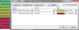
  2. How to use the “Sort by Colors” feature introduced in Excel 2007.
  3. How to add a Check Box Form Control that will “toggle” the Conditional Formatting On or Off.

Paste Special “Live Preview”

I demonstrate a great new feature introduced in Excel 2010, “Live Preview” for Paste Special. You will use Paste Special – Formats to extend the rules for Conditional Formatting to a new range of Cells

Sort by Color

Beginning with Excel 2007, you can now sort fields based upon the color of a font or a cell background. I show how this works.

The Check Box Form Control

The “key concept” to understand when using Excel’s Form Controls is the “Cell Link.” With a Check Box Control, the value in the Cell Link is TRUE when the box is “checked” while the value is FALSE when it is Unchecked. We can use this information to create a “Conditional Format based upon a Formula.”

Conditional Formatting Rules

When you base Conditional Formatting upon a Formula, the result of that formula must return TRUE in order apply this formatting. Setting the background cell color to “White” effectively “hides” the previous background cell colors.

Shop for The 50 Best Tips for Excel 2007

Shop for The 50 Best Tips for Excel 2007

Resources Offered for Sale

I encourage you to visit my secure online shopping website – http://shop.thecompanyrocks.com – to preview the many training resources that I offer you. Check out my latest Excel Training Videos:

Watch this Video in High Definition

Click on this link to watch this video in High Definition on my YouTube Channel – DannyRocksExcels


How to Use Structured Formula References for Tables in Excel 2007 and Excel 2010

Structured Formula Reference - Excel 2007

Structured Formula Reference - Excel 2007

Beginning with Excel 2007, you can – and should – convert a Standard Data Range to an Excel Table. Doing so offers several advantages:

  • You get a selection of Table Styles – including Alternate Row Shading – that make it easier to read your tables.
  • You can automatically extend the Scope of your Table – by adding additional Fields (Columns) or Records (Rows).
  • You can give your Table a “Name” to reflect the purpose of the Table.
  • You can add a Total Row to Subtotal each Field (Column) and you can change the Function used to Subtotal from a drop-down menu.
  • You can apply Structured Formula References in the Table – Enter the Formula in a Single Cell and it is Automatically copied down for each record in the Table.

“In This Row” Formula Styles

Structured Formula References use a new style of formulas. Rather than referring to a specific Cell, in an Excel Table, you refer to a Field “in this row.” This type of formula is easy to create “inside the table.” It is also fairly easy to create “outside the Table” using the new Formula AutoComplete tool. You will be using [ ] (Left & Right Brackets) for these formulas. I go over these details, in-depth, in this video tutorial.

There are also distinct differences in how Structured Formula References are created between Excel 2007 and Excel 2010. These Structured Formula References are greatly streamlined in Excel 2010 – in my opinion.

The SUBTOTAL() Function and Excel Tables

I strongly recommend that you become familiar with how to use the valuable SUBTOTAL() Function in Excel when referring to the data in a Table. With the SUBTOTAL Function, you can produce a wide range of summaries anywhere on your Excel Workbook. And… the Subtotal Results reflect the totals for any “Filters” that you apply to your Table.

Play this Video in High Definition

Watch this Video in High Definition

Follow this link to watch this Excel Tutorial in High Definition on my YouTube Channel – DannyRocksExcels

Go to Part 2 in this Series of Tutorials

Follow this link to go to Part 2 in this series of tutorials about using Structured Formula References in Excel Tables.

Announcing 6 New Products on My New Online Secure Shopping Website

I invite you to visit my new online shopping site. I have added 6 new products – Extended Length Video tutorials that you can either “download now” or purchase as a DVD-ROM. Each product contains over 90 minutes of in-depth video instruction for Pivot Tables. You can choose the product to fit your version of Excel – Separate products for Excel 2003, Excel 2007 and Excel 2010.

Click here to view my new products.

How to Customize the Quick Access Toolbar in Excel 2007

Quick Access Toolbar Office 2007

QUick Access Toolbar in Office 2007

Learning how to Customize the Quick Access Toolbar (QAT) in Excel 2007 or Excel 2010 is a great way to ease the “learning curve” when you upgrade versions.

In my experience, I have found that most people do not even realize that there is a Toolbar in Excel 2007, let alone that you can move it to a different location and to customize it!

What I Cover in this Video Tutorial

Here is what you will learn from this YouTube Video Tutorial:

  • To move the QAT to Show it Below the Ribbon (recommended!)
  • To add the most popular command buttons one at a time
  • To open the Customize Quick Access Toolbar Dialog Box
  • To find commands to add – including Command Not in the Ribbon!
  • To organize the commands on your QAT
  • To create a customized QAT for “specific workbooks”  – great for special projects!
  • To quickly add individual command buttons with a right-click of the mours
  • To add entire command button groups to the QAT with a right-click of the mouse – (recommended!)

Since this video is a little longer than usual, I am making it available exclusively on my YouTube Channel.

Watch Video in High Definition Mode

Follow this Link to view this tutorial in High Definition on my YouTube Channel – DannyRocksExcels

“The 50 Best Tips for Excel 2007” DVD-ROM

Purchase my DVD-ROM, “The 50 Best Tips for Excel 2007” – on sale now at http://shop.thecompanyrocks.com for only $29.97 USD!

Tips to Help You Remain Productive When Upgrading to Excel 2007

Beginning Level Videos for Excel

Videos at the Beginning Level - 50 Best Tips for Excel

I enjoy participating in several discussion and sharing groups on LinkedIn. In one group, the question was raised, “The Ribbon – Love it or Leave it?” Many group members wrote to say that they just cannot figure out the new user interface – The Ribbon. Others expressed frustration that they were much less productive in their work as they tried to make the transition to either Excel 2007 or Excel 2010. Some said that they simply gave up and returned to using Excel 2003.

Certainly, I felt frustrated and lost when I first began to use Excel 2007. So, let me share my best tips for quickly adjusting to and mastering the commands and tools in Excel 2007 – and Excel 2010.

Topics Covered in this Video

  • The Office Button in Excel 2007 to open, save and print Excel workbooks and to change Excel Options
  • 7 Standard Tabs on the Ribbon
  • Groups of related Command Buttons
  • Launchers to open up Dialog Boxes
  • Command Buttons with Menus
  • Showing the Quick Access Toolbar below the Ribbon
  • Customizing the Quick Access Toolbar
  • Working with the Mini Toolbar

Watch Video in High Definition on YouTube

Follow this link to watch this Excel Video Tutorial in High Definition on my YouTube Channel – DannyRocksExcels

Purchase My DVD-ROM, “The 50 Best Tips for Excel 2007”

Here is the link to learn more about my best-selling DVD-ROM. You can purchase this from my online store using a secure shopping cart. On sale now for only $29.97 USD.


Three and a Half Ways to Average Excel Data Using Criteria

AverageIf Function in Excel

AverageIf Function in Excel

It is easy to use Excel’s AVERAGE Function to get the average for an entire range of data. But, what if you are asked to produce a report that shows the average for select groups of records – for example, average test results for the female students only; or for the male students only? What approach do you take? What Functions do you use to produce this report?

Three and a Half Ways to Produce this Report

  • SUBTOTALS – Easy to use. Remember to sort your data first using the field that you want to subtotal.
  • AVERAGEIF Function – Very easy to use. Only works in Excel 2007 and Excel 2010.
  • DAVERAGE Function – Will work in any version of Excel. Easy to add or change the Criteria.
  • PIVOT TABLE – Very easy to create. No need to write a formula. Create report with @ 6 mouse clicks!

My Preferred Approach – Create a Pivot Table Report

While Pivot Tables are the most powerful tool in Excel, they are also one of the easiest tools to use in Excel! Why?

  • Because you can create a Pivot Table Report without writing a single formula!
  • You can create this Pivot Table Report with about six clicks of the mouse.
  • You cannot possibly harm your underlying data when you create Pivot Tables!

Download a One Hour- Plus / In-depth Video Tutorial on Pivot Tables – for $9.95

I have created a series of Excel Video Tutorials that you can download for $9.95 US Dollars each. Here is a link to my informational page that gives you the details.

  • Are you Using Excel 2003? – I created a video recording for Pivot Tables using Excel 2003 that you can download for $9.95!
  • Are you Using Excel 2007? – I created a video recording for Pivot Tables using Excel 2007 that you can download for $9.95!
  • Are you Using Excel 2010? – I created a video recording for Pivot Tables using Excel 2010 that you can download for $9.95!

As with all of my products, I guarantee that you will be 100% Satisfied or I will refund your purchase price – no questions asked!

My Extended length Excel Training Video Recordings are hosted at: http://thecompanyrocks.webex.com – I use the secure shopping cart at WebEx by Cisco Systems, so you can be sure that your personal information is safe and secure.

Watch Video in High Definition on YouTube

Follow this link to watch this video tutorial in High Definition mode on my YouTube Channel – DannyRocks Excels

Get My DVD-ROM, “The 50 Best Tips for Excel 2007” for only $29.97

Download My 75 Minute Video Tutorial on Excel 2007 Pivot Tables

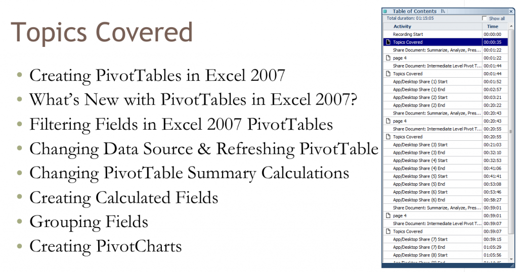
Topics Covered

Table of Contents for Recording

I have just recorded and published a 75 Minute Video Tutorial titled, “How to Create and Modify a Pivot Table in Excel 2007 to Summarize, Analyze and Present the Information in your Data Set.”

It is published on my WebEx by Cisco site: http://thecompanyrocks.webex.com Follow this link to go directly to this recording.

There is a charge for this recording – US$9.95 In addition to the recording you get:

  • A Step-by-step instructional manual
  • Access to the Excel workbook files that I used for this recording

Not to brag , but I think that this video tutorial is excellent! I spent many hours planning out the exercises, working through the timing of each chapter of the video and practicing my delivery. I am happy with the result. And, more important, I think that you will also be satisfied with what you will learn from this recording!

What You Will Learn on My Recording

My goal is to give you a comprehensive understanding of Excel 2007 Pivot Tables. But to give you the opportunity to learn this in “bite-size chunks” that can replay when necessary. I created realistic exercises to illustrate each topic.  Also notice that I have created a Table of Contents for the recording so that you can go to a specific chapter on the recording. You can stop and start at any point.

How to Download this Recording

  1. Go to http://thecompanyrocks.webex.com or click on this link to go to the main menu.
  2. Click on “Recorded Sessions.”
  3. Click the link for the recording, “Excel 2007 Pivot Tables to Summarize Data.”
  4. Register for this session (First Name, Last Name and email address).
  5. Enter payment information (PayPal or Credit Card). This is a secure site!
  6. Follow the instructions to Download my recording.
  7. Recommended – you can also download the ARF Recorder to view the recording.
  8. At this point you can decide to convert the recording to a different format. E.g. WMV (Windows Media Player), SWF (Flash) or MP4 (MPEG4)
  9. At the end of the recording, you are taken to a web page with links to download the Instructional Manual and to download the Excel Workbook that I used during this recoring.

Give Me Your Feedback

I welcome your comments and suggestions for future video tutorial recordings. You can add your comments below or send them to me via email.

How to Convert a Pivot Table to a Standard List

Watch this video tutorial in High Definition on YouTube

A viewer aksed for my help. She has a boss and a few customers who:

  1. Do not know how to create or use Pivot Tables
  2. Have no desire to learn how to create and use Pivot Tables
Convert Pivot Table to Standard List

Convert Pivot Table to List

Nevertheless, in this example, she is being asked to create a summary report – by Year and by Quarter – from @ 5,000 daily transaction records. The fastest way to create this report is with a Pivot Table. Now, to meet the demands of her boss and clients, she needs to convert this Pivot Table into a standard list that can be Filtered and Subtotaled.

Summarize by Year and Quarter

To create this Pivot Table report:

  • Add the “Date” field to the grid and then select a single date.
  • Group the Date field by Month, Quarter and Year.
  • Add and arrange the Customer and Invoice fields to the Pivot Table Grid.

Convert Pivot Table to Standard List

  1. Remove both the Subtotals and Grand Totals from the Pivot Table Report.
  2. In Excel 2007 & 2010, ensure that you are using either the Outline or Tabular report layouts – NOT the new “default” Compact layout.
  3. Also in Excel 2007 & 2010, remove the Field Headers and the + / – Symbols.
  4. Now, select the entire Pivot talbe (use Ctrl + A) and copy it to the clipboard.
  5. Use Paste Special Values to paste the Pivot Table Results.

Filling the Blank Cells in the List

As you can see, whenever you have “nested rows” in a Pivot Table you get a nice, clean report. However, in order to Filter and Subtotal this new list, you will need to “fill in the blank cells.”

  1. Select all of the values and all of the blanks in Column A.
  2. Use Ctrl + G (or F5) to open the Go To Dialog Box and choose Special.
  3. From the Go To Special choices choose “Blanks.”
  4. With all of the Blank Cells selected use this formula: = ↑
  5. Do NOT press Enter. Rather, press Ctrl + Enter and all of the Blank Cells are now filled in with the Customer Names!
  6. Finally use Copy, Paste Special, Values to complete this process.

Watch This Video on My YouTube Channel – DannyRocksExcels

Since this video tutorial is a little longer than usual, I have decided to post it as a video – in High Definition – on my YouTube Channel. Click here to view it or copy and paste this link into your browser:

Link to YouTube Video:   http://youtu.be/IwReVDJ7BAI?hd=1

Download This Excel Workbook

Learn How to Quickly Create Excel Pivot Table Reports

Excel Data Set

Data Set in Excel

Many people are curious about Excel Pivot Tables. They would like to learn how to create a Pivot Table, but they fear that that will take too long and be difficult to learn. 

Here’s the good news! Pivot Tables are one of the most powerful tool in Excel AND Pivot Tables are also one of the easiest Excel Techniques to learn! It sounds like a contradiction, doesn’t it? 

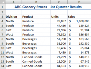
How would you like to turn this data set – with over 500 rows of data … 

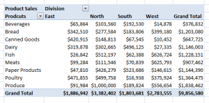
into this Pivot Table Summary Report with @ six clicks of the mouse? 

Pivot Table Row & Column

Pivot Table Summary

 That’s all it takes. With a Pivot Table you turn long lists of data into summarized information that highlights the trends and patterns in your business. 

Special: Save 20% on any purchase! Use Coupon SAVE-20-PCT during Checkout! 

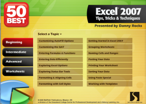
I can teach you how to get started on the road to mastering Excel Pivot Tables. On my DVD-ROM, “The 50 Best Tips for Excel 2007,” I have the following Pivot Table video lessons: 

  • Introducing Pivot Tables – Run time: 8:23
    • Why Use Pivot Tables?
    • How to Create a Pivot Table
    • How to Modify a Pivot Table
    • How to Update a Pivot Table
  • Grouping and Charting in Pivot Tables – Run time: 5:50
    • Grouping Pivot Table Fields by Month, Quarter and Year
    • Grouping Pivot Table Fields by Week
    • Collapsing and Expanding Pivot Table Fields
    • Creating Pivot Charts
  • Using New Pivot Table Features in Excel 2007 – Run time: 7:46
    • Base Your Pivot Table on an Excel Table
    • Adjust Pivot Table Report Layouts
    • Apply Conditional Formatting to Pivot Tables
    • Insert Blank Rows in Your Pivot Table Report
The 50 Best Tips

The 50 Best Tips Series

As you can see from the “Run times,” each lesson is focused on one Excel technique. If you don’t have a lot of time and you want to quickly learn how to create Pivot Tables, my DVD-ROM is the best place to begin. 

Here is a PDF that you can download to see the content and Run times for each of my tips: The 50 Best Tips for Excel 2007 Detailed Content Listing 

And, here is a link to my Archive of Free Pivot Table Videos  on The Company Rocks website. 

Learn how to “Quickly Create Excel Pivot Table Reports and Charts” 

Thank you! 

Danny Rocks

Use the SUMPRODUCT Function to Total Lists Using Multiple Criteria

In Excel 2007 and Excel 2010 you can use the new SUMIFS Function to total a list using multiple criteria. This is a great new feature!

But … what if you are using Excel 2003 or earlier? Or, if you collaborate with colleagues and clients who use older versions of Excel – how can you use multiple criteria to select the records that you want to Sum? You can use the SUMPRODUCT Function as I demonstrate in this video lesson.

The 50 Best Tips

The 50 Best Tips Series

Key Concepts

  • Create – and use – Named Cell References for Ranges / Arrays in your formulas
  • Use the Function Arguments Dialog Box – Use the keyboard shortcut Ctrl + A to bring this up
  • Use the F3 Keyboard Shortcut to bring up the Named Ranges List
  • In this lesson, use () to enclose each Array Argument
  • In this lesson, use * to substitute for the , to separate each Array in the formula (Edit this in the Formula Bar)

There are usually several ways to solve any problem in Excel. This is a good procedure to learn – regardless of the version of Excel that you use.

Click here to view the 1st part of this series on how to use the SUMPRODUCT Function in Excel.

You can view this Excel Video in Hig Definition, Full Screen Mode on my YouTube Channel – DannyRocksExcels by clicking here.

I cover the SUMIF and SUMIFS Functions in greater detail on my DVD, “The 50 Best Tips for Excel 2007.” Click here to start shopping using my secure shopping cart.

Learn how to “Master Excel in Minutes – Not Months!”

My Most Viewed and Downloaded Videos for Excel and PowerPoint

My iTunes Podcast

Danny on iTunes

I began to post my videos as podcasts at the iTunes store this past summer. Since then, my video lessons for Excel and PowerPoint have been viewed and downloaded many times. I am thirlled. And, I thank you for your support and encouragement.

Here are the links – on my website – to the most popular video episodes. I have organized them by category in the order of their popularity. You can click on any link to view or download that video from my website. Or, you can go to my video Podcast by clicking on this link – “Danny Rocks Tips and Timesavers” Podcast on iTunes.

Merging and Consolidating Excel Worksheets

 PowerPoint Presentations

Data Visualizations

What-If Analysis in Excel

Importing Data From Other Programs

Pivot Tables

Excel Tables

Social Media

Formula Errors

Please add your comments below – or on my iTunes Channel. I welcome your feedback.

You can learn how to “Master Excel in Minutes – Not Months!”

Sincerely,

Danny Rocks