Use an Excel Template to Customize a Worksheet with 52 Weeks of Employee Time Cards

Template for Time Cards in Excel

Time Card Templates in Excel

This is Part Two in my new series of Excel Tutorials where I share my best practice tips for creating 52 weeks of Employee Time Cards – for hours worked. In this segment, I focus on starting the process with an Excel Template.

Finding Templates for Time Cards

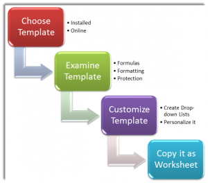
As I demonstrate in the video, there are at least two easy sources for finding a Time Card Template:

  1. Sample Templates Installed on your Computer
  2. Templates that you can preview and download from the Microsoft Office Templates Website

Examining Templates that You Download

Before you even think about duplicating the Excel Template that you just downloaded, it is important for you to take a few minutes to explore:

  • The Formulas used in the Template
  • The Formatting used in the Template – especially the formatting for Dates and Times
  • The Protection Applied (if any) to the cells or the entire worksheet

Creating Drop-down Menus for your Template

Since our premise here is that we will copy the template to 51 additional worksheets, it makes sense to use Data Validation to create a series of “drop-down menus” for Employee names and the Start Date for each week. I demonstrate how to do this in the video tutorial.

Links to Additional Video Tutorials in this Series

Additional Resources for Excel

I invite you to visit my new, secure, online shopping website – http://shop.thecompanyrocks.com – to discover the many training resources that I offer you!

Watch Tutorial in High Definition

Follow this link to watch this Excel Tutorial in High Definition on my YouTube Channel – DannyRocksExcels
Click to Watch Video Now

Tips for Creating 52 Weeks of Employee Time Cards in Excel

Insert & Copy Worksheets

Insert & Copy Worksheets

We are now winding down the end of the year 2011. Several of my viewers and clients have asked my for help in creating one Excel Workbook that will contain 52 weeks of employee time card information:

  • Name and Department of Employee
  • Hours Worked each day of the week – Regular and Overtime
  • Number of Holiday / Sick Days that were used / that remain, etc.

First Tutorial in this Series

Rather than trying to create each individual – and some are very specific – request, I have decided to combine multiple requests into a series of Best Practice Tips for my general audience to consider.

In this lesson, I demonstrate:

  • Two methods for adding new blank worksheets to the Excel workbook
  • Two Methods for inserting an exact copy of an existing – and formatted – worksheet
  • My favorite tip – Fill Across Worksheets – either the formatting only, the contents only or the default setting – both formatting and contents.

Links to Additional Tutorials in this Series

Watch Tutorial In High Definition

Follow this link to watch this tutorial in High Definition on my YouTube Channel – DannyRocksExcels

Additional Resources at My Online Shopping Website

I invite you to visit my new – secure – online shopping website – http://shop.thecompanyrocks.com – and preview the many tutorials and resources that I offer you.

Watch Tutorial Now

How to Use the New Natural Language Date Filters in Excel

Natural Language Date Filters

Natural Language Date Filters

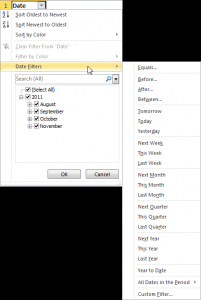
Recently, one of my viewers asked me to go into greater detail in demonstrating how the new Natural Language Date Filters work in Excel. Natural Language Filters were introduced in Excel 2007 and they are a great tool to use! Now, instead of writing complex formulas as criteria in Advanced Filters, you can simply click, “Yesterday” to see all of the records from the previous day!

Of course, you must actually have records in your data set for that date!

The Natural Language Date Filters are related, by position, to TODAY(). The TODAY() Function is a “Volatile Function” that returns the value for the current date as found in your computer systems internal clock. The result of the TODAY() Function will change each day. And so, by definition, will the result for a “Yesterday” filter!

Filter for Specific Date

There are several methods that you can use to filter for a specific date or range of dates. One method that I demonstrate in this tutorial is the “Custom Date” dialog box.

Watch Tutorial in High Definition

Follow this link to watch this Excel Tutorial in High Definition on my YouTube Channel – DannyRocksExcels
Learn About My New Extended Length Video Tutorials

I have recently released a series of extended length (90 minutes) video tutorials. They are part of my “Master Excel in Minutes” Series. Each video focuses on one topic. My first video is focused on Excel Pivot Tables. I have created Videos for Excel 2010, Excel 2007 and for Excel 2003. You also have the choice of purchasing the video for immediate downloading or shipped to you on a DVD-ROM.

Follow this link to go to the information page for my “Master Excel in Minutes” video tutorial series.

Keyboard Shortcuts to Enter and Edit Data Efficiently in Excel


Keyboard Shortcuts to Enter Data

Keyboard Shortcuts to Enter Data

This is the latest installment in my series of video tutorials where I demonstrate how to use Keyboard Shortcuts in Excel. In this tutorial, I demonstrate how to Enter and Edit Data Efficiently in Excel using Keyboard Shortcuts.

Tips Covered on Video Tutorial

Here are the main Keyboard Shortcuts that I show you how to use on this video:

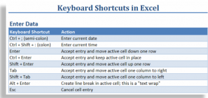
  • Enter Current Date in a cell.
  • Enter Current Time in a cell.
  • Use Ctrl + Enter to accept data entry and keep the focus on the current cell.
  • Use Ctrl + Enter to populate a range of selected cells.
  • Use Alt + Enter to “Wrap the Text” in a cell.
  • Use F2 to edit data inside a cell.
  • Use Ctrl + left & right directional arrows to move to the beginning of the next / previous word while editing in the cell.
  • Use ‘ (apostrophe) as the first character in a cell to make this a “text” entry.

Download my complete Chart of Popular Keyboard Shortcuts as a PDF 

 Follow this link to download – for free – my 5 Page Chart of Popular Excel Keyboard Shortcuts as a PDF.

Subscribe to my Video Podcast on iTunes

Here is the link to subscribe to my video podcast, “Danny Rocks Tips and Timesavers” on iTunes. It is offered for free!

Watch Tutorial in High Definition on YouTube

Follow this link to view this Excel Tutorial in High Definition mode on my YouTube Channel – DannyRocksExcels

How to Use Excel Keyboard Shortcuts to Cut, Copy and Paste Formulas and Formatting

Keyboard Shortcuts for Cut, Copy & Paste

Keyboard Shortcuts for Cut, Copy & Paste

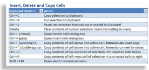
In addition to showing you the Keyboard Shortcuts to Cut, Copy and Paste in Excel, I demonstrate how these actions affect formulas and formatting.

Topics in this Tutorial

Here are the topics that I demonstrate in this video tutorial:

  • Select multiple cells using the keyboard
  • Use Ctrl + Enter to update all cells in the selection
  • Use Ctrl + ~ to “toggle” between showing and hiding formulas in all cells
  • Use F2 to edit in the cell – and to diagram cell references for formulas
  • Use Ctrl + C to copy the “relative cell references” in a formula
  • Use Ctrl + X to cut an Excel formula that retains the original cell references
  • Open and use the Office Clipboard to store up to 24 most recent copy and cut items
  • Use Ctrl + Z to undo multiple actions
  • Use Ctrl + A to select all cells in a contiguous range
  • Use the Delete key to delete the contents of a cell or range while retaining the formatting
  • Use the Clear All command to remove both formatting and contents in a range of cells

Download My Complete Charts of Popular Keyboard Shortcuts

Follow this link to my Excelusive Membership Content Page where you can download all of my charts and tables of Keyboard Shortcuts.

Watch Video in High Definition

Follow this link to view this tutorial in High Definition on my YouTube Channel – DannyRocksExcels
How to Use Keyboard Shortcuts in Excel to Control Basic File Operations

Excel 2007 File Operations

Excel 2007 File Operations

If you have recently upgraded to either Excel 2007 or Excel 2010, you REALLY NEED to master the Keyboard Shortcuts that I present in this lesson!

Many Excel veterans who upgrade, tell me that they initially felt “lost” with the new user interface. Some of my clients called me in a panic because they didn’t know where to look to Print their work or to open a document. If you know how to use the Keyboard Shortcuts that I present in this lesson, you will never be at a loss. As an added bonus, these Keyboard Shortcuts work with ALL Microsoft Office programs and also for most Windows-based programs.

The “N-O-W-S” Keyboard Shortcuts

I use this acronym – NOWS – to remember the keyboard shortcuts to Open, Close and Save Documents in MS Office programs. Use Ctrl + W to Close the active worksheet.

In this video tutorial, I also show you when NOT to use Keyboard Shortcuts! There are many times when you need to access the full file menu selection.

Keyboard Shortcut for Print Preview

Use Ctrl + F2 to open up the Print Preview pane. Use the “Esc” key to Exit Print Preview.

Download My Chart of Popular Keyboard Shortcuts as a PDF

Follow this link to go to the web page where I store my Keyboard Shortcut Charts and other download-able content.

These Keyboard Shortcuts work for all versions of Excel. So far, I have found only one Keyboard Shortcut that is different when used in Excel 2007 / 2010 than in Excel 2003.

More Video Tutorials for Keyboard Shortcuts

This is the first in a series of video tutorials that I have planned. Each video will focus on the Keyboard Shortcuts you can use to perform a specific task – e.g. Formatting Cells, Inserting and Deleting, etc. My plan is to post one new video in this series per week.

Watch Video Tutorial in High Definition Mode

Follow this link to view this video tutorial in High Definition on my YouTube Channel – DannyRocksExcels


How to Customize the Quick Access Toolbar in Excel 2007

Quick Access Toolbar Office 2007

QUick Access Toolbar in Office 2007

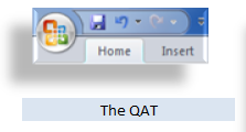
Learning how to Customize the Quick Access Toolbar (QAT) in Excel 2007 or Excel 2010 is a great way to ease the “learning curve” when you upgrade versions.

In my experience, I have found that most people do not even realize that there is a Toolbar in Excel 2007, let alone that you can move it to a different location and to customize it!

What I Cover in this Video Tutorial

Here is what you will learn from this YouTube Video Tutorial:

  • To move the QAT to Show it Below the Ribbon (recommended!)
  • To add the most popular command buttons one at a time
  • To open the Customize Quick Access Toolbar Dialog Box
  • To find commands to add – including Command Not in the Ribbon!
  • To organize the commands on your QAT
  • To create a customized QAT for “specific workbooks”  – great for special projects!
  • To quickly add individual command buttons with a right-click of the mours
  • To add entire command button groups to the QAT with a right-click of the mouse – (recommended!)

Since this video is a little longer than usual, I am making it available exclusively on my YouTube Channel.

Watch Video in High Definition Mode

Follow this Link to view this tutorial in High Definition on my YouTube Channel – DannyRocksExcels
“The 50 Best Tips for Excel 2007” DVD-ROM

Purchase my DVD-ROM, “The 50 Best Tips for Excel 2007” – on sale now at http://shop.thecompanyrocks.com for only $29.97 USD!

Tips to Help You Remain Productive When Upgrading to Excel 2007

Beginning Level Videos for Excel

Videos at the Beginning Level - 50 Best Tips for Excel

I enjoy participating in several discussion and sharing groups on LinkedIn. In one group, the question was raised, “The Ribbon – Love it or Leave it?” Many group members wrote to say that they just cannot figure out the new user interface – The Ribbon. Others expressed frustration that they were much less productive in their work as they tried to make the transition to either Excel 2007 or Excel 2010. Some said that they simply gave up and returned to using Excel 2003.

Certainly, I felt frustrated and lost when I first began to use Excel 2007. So, let me share my best tips for quickly adjusting to and mastering the commands and tools in Excel 2007 – and Excel 2010.

Topics Covered in this Video

  • The Office Button in Excel 2007 to open, save and print Excel workbooks and to change Excel Options
  • 7 Standard Tabs on the Ribbon
  • Groups of related Command Buttons
  • Launchers to open up Dialog Boxes
  • Command Buttons with Menus
  • Showing the Quick Access Toolbar below the Ribbon
  • Customizing the Quick Access Toolbar
  • Working with the Mini Toolbar

Watch Video in High Definition on YouTube

Follow this link to watch this Excel Video Tutorial in High Definition on my YouTube Channel – DannyRocksExcels

Purchase My DVD-ROM, “The 50 Best Tips for Excel 2007”

Here is the link to learn more about my best-selling DVD-ROM. You can purchase this from my online store using a secure shopping cart. On sale now for only $29.97 USD.


Working with Custom Lists in All Versions of Excel

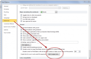
Edit Custom Lists in Excel

Edit Custom Lists in Excel

Custom Lists in Excel are great because the help to ensure accuracy and consistency when entering data on a worksheet. Excel comes with several Custom Lists built-in to the program – e.g. Days of the Week and Months of the Year. Now, you can quickly use Excel’s AutoFill handle to add Jan, Feb, Mar, Apr, etc. in any direction (vertical or horizontal) on the active worksheet.

Edit Custom Lists

You can quickly create – or edit – your own Custom List. Follow these steps:

  1. Type your list in a contiguous group of cells – either vertically or horizontally.
  2. Select the cells with the values that you just entered.
  3. Spell check this list – use the F7 Keyboard Shortcut
  4. Open up the Edit Custom List Dialog Box. (Watch this video to see how this is differs between Excel 2010, Excel 2007 and Excel 2003.)
  5. With your new Custom List selected, click the “Import” button to add your Custom List to the current version of Excel on this computer.

Sort Data Using a Custom List

On this video tutorial, I demonstrate how to sort a list of data using a Custom List – e.g. to get the “Month” field sorted in chronological order (January, February, etc.) This will save you a great deal of time!

Create a Custom List for Letters of Alphabet

Having a Custom List for the 26 letters of the alphabet comes in handy on many occasions. I show you how to AutoFill down the initial list using =Char(Row() + 64) beginning in Row 1 – a really usefuly function!

View This Excel Video Tutorial in High Definition

Follow this link to watch this video tutorial in High Definition on my YouTube Channel – DannyRocksExcels
Get my best-selling DVD-ROM, “The 50 Best Tips for Excel 2007” for only $29.97!

Make it Easier to Display Large Numbers in Excel with Formatting Codes

In order to establish and maintain your credibility, the numbers that you store in Excel must be accurate and precise. You cannot compromise on this principle! In most cases, you will be working with large numbers – sometimes, very large numbers. And, this may present a problem when you need to present these numbers to your audience.

So …

It is essential that you distinguish between your need to maintain accurate “data” and your need to communicate the essential “information” that resides in your data to your audience.

Format Custom Numbers

Format Custom Numbers in Excel

When you are presenting the “essential information” that resides inside your database, you need to consider the needs of your audience.

Ask yourself these questions:

  • What essential information do you need to communicate to your audience?
  • What are the trends and variances that you see inside your data, that you want your audience to see, to understand, and take action on?
  • What level of precision do you need to convey to your audience so that they can grasp this information?
  • How can you make it easier for your audience to see – and understand – the trends and variances in your data?
  • What techniques can you use to present this information to your audience?

Apply a Custom Format to Numbers in Excel

You can answer these questions by learning how to apply “Custom Number Formatting” in Excel.

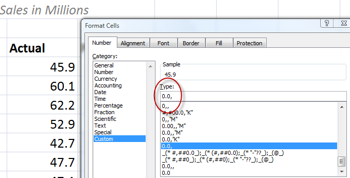
For example, instead of presenting this level of precision – 19, 699, 499, you can use this custom number format – 0.0,,”M”, to present this as 19.7M. From my perspective as both a presenter and an audience member, I prefer to see 19.7M. This makes it easier for me to process the information as an audience member. This makes it easier for me to present – saying 19,7 million is a lot easier than trying to say 19 million, 699 thousand, 4hundread and 99 dollars!

What is your preference?

Watch this short, focused Excel training video lesson to learn how to format and display large numbers in Excel so that you can make it easier for your audience to understand and act on the information that you are presenting.

Learn how to “Master Excel in Minutes – Not Months!”

Follow this link to watch this video lesson in High Definition, Full-screen mode on my YouTube Channel – DannyRocksExcels