How to Use Date Functions and Date Formatting in Excel

In this lesson, I respond to two recent requests from viewers for help in Using DATE Functions in Excel and also, how to apply Custom Date Formatting. I get similar requests on a frequent basis from both viewers and clients.

Solve Problem #1 

My first viewer wants help in using the DATE() Function in Excel. She wants to calculate a date that is 90 days after the starting date for a project. She encountered two problems

  1. Initially, the DATE() Function produced and error – because she forgot to ‘nest” the YEAR(), MONTH()+9, DAY() Functions inside the DATE() Function.
  2. She was not expecting a date to be filled in the formulas column when there was no starting date for the project – She needed to include an IF() function to perform a LOGICAL TEST – Does  the Starting Date = 0, Value if TURE, ” ” (to display nothing), Value if FALSE – to perform the calculation.
Excel Custom Date Formats

Excel Custom Date Formats

Solve Problem #2

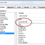
My second viewer wanted my help to ensure that the date values that he “pasted” into a range of cells were in the (Custom) format of “yyyy-mm-dd” (Year, Month, Date).

In this case, we need to take two steps:

  1. Format the destination cells using the CUSTOM FORMAT of yyyy-mm-dd that we create.
  2. After “Pasting” the Copied Cells, use the “Paste Options” dialog box to select – “Match Destination Formatting.”

I also demonstrate how to use the NETWORKDAYS() Function and the WORKDAY() Function – with an optional list of “Holidays” to exclude. And, finally, I show you the “pitfalls” that occur when you import a “text” file of dates that use a variety of formats. In order to perform DATE calculations, a date must be stored as a NUMBER in Excel. It must be right-aligned in the cell.

You can watch this Excel Video Lesson in High Definition, Full Screen Mode on my YouTube Channel – DannyRocksExcel – by clicking this link.

Learn to “Master Excel in Minutes – Not Months!”

How to Use Conditional Formatting to Compare Two Excel Lists

Clients and viewers frequently ask me to help them to compare two differeny lists in Excel. They want to find – or highlight – the values that are different in each list. For example, which customers appear in the 1st list but NOT in the 2nd list. So, I created this video lesson to demonstrate how to do this with Conditional Formatting.

In an earlier Excel Video Lesson, I demonstrated how to compare two Excel lists using either the MATCH() Function or the VLOOKUP() Function.

Conditional Formatting Rule

Conditional Formatting Rule

Use Conditional Formatting

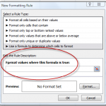
I demonstrate how to use Conditional Formatting to Highlight the Cell Values that are different when you compare two Excel Lists. I will use a “New Rule with a Formula” that must return the answer TRUE, to trigger the special formatting.

In Conditional Formatting, you first establish a “condition” that can be answered as either TRUE or FALSE. Then, for those cells where the answer to the condition is TRUE. the special “cell formatting” that you chose will apply.

In this lesson we will be using this Formula: =COUNTIF(List 2, 1st cell in List 1) = 0.

Steps to follow:

  1. Select the cells that you want the Conditional Formatting to apply to- in our example List 1.
  2. On the Home Tab of the Ribbon, click the Conditional Formatting arrow and select New Rule.
  3. Select New Rule – “Use a Formula to determine which cells to format.”
  4. Enter the formula – e.g. =COUNTIF(Range, Criteria) = 0 where the “Range” is the list of values in List 2 (Absolute Reference) and the “Criteria” is the 1st cell reference in List 1 (Relative Reference).
  5. Choose the Format for the cells when the condition is met – the result is TRUE. In this example, I choose to “FILL” the cells with a Blue background color.

Want to watch this video in High Definition, Full-Screen Mode? Click here to go to my YouTube Channel, DannyRocksExcels

Learn to “Master Excel in Minutes – Not Months!”

How to Calculate Overtime and Standard Hours Worked on a Time Card in Excel

One of my viewers asked me to show him how to calculate the number of hours worked each day – separated by standard hours and by overtime hours. He, like many Excel users, is frustrated when performing calculations involving time. They create a standard formula, but the results are not what they were expecting. In most cases, this is because of the need to FORMAT the cells that contain calculations to accommodate Excel’s logic.

Excel Time Card

Excel Time Card

Time Functions and Formats

In this lesson, I demonstrate the following functions and formats:

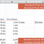
  • The =TIME() Function requires three arguments (Hours, Minutes, Seconds). In this example, I use =TIME(8,0,0) in a cell to represent the Standard Hours Worked each day – i.e. 8 hours.
  • The CUSTOM Format h:mm to format the cells that contain the results of time calculations (Total Hours Worked each day, Regular and Overtime Hours Worked each day).
  • The CUSTOM Format [h]:mm to format the cells that contain the results of SUM() for the Total Hours, Regular and Overtime Hours Worked each WEEK – i.e. Hours that exceed 24 hours
  • The Formula =SUM(Overtime Hours Worked this week) * 24 to gives me the NUMBER equivalent – Remember to format this cell as a NUMBER – not as [h]:mm,  so that you can multiply it by the cell that contains the Hourly Rate that you pay for either Regular Hours or Overtime Hours.

How Time is Stored vs. How Time is Displayed

Remember to distinguish between what Excel Stores as a calculation and how Excel Displays the result of a calculation. This is especially important with TIME and DATE Calculations in Excel.

You can view this lesson in High Defintion, Full Screen Mode on my YouTube Channel – DannyRocksExcels – by clicking this link.

I invite you to subscribe to my free Video Podcast – “Danny Rocks Tips and Timesavers”- at the iTune Store by clicking here.

Vist my Online Shopping Site

My DVD-ROM, “The 50 Best Tips for Excel 2007” is on sale at my Online Bookstore – http://shop.thecompanyrocks.com –  Click here to open a secure shopping cart.

Learn how to “Master Excel in Minutes – Not Months”

How to Import Excel Data Into Access

This is the first in a series of lessons where I demonstrate how to integrate Excel data with an Access database. In this lesson you will learn how to:

  • Access Working with External Data

    Work with External Data

  • Import an Excel worksheet as a new Table in Access.
  • Append an Excel worksheet to the Table that we created with the Imported data.
  • Create a link between the Source Excel worksheet and an Access Table.
  • Refresh the link between Excel and Access.

First, on the Excel side of this process, make sure that you have clearly identified the Field Headers in the Top Row of your data set. If you have and cells that contain Formulas, convert the formulas to Cell Values.

Begin the Import Process

You initiate the Importing from inside Access. Go to the External Data tab on the Ribbon (in Access 2007) and choose Excel. Follow the steps in the Import Wizard. I recommend that you allow Access to create a Primary Key for the new table. This will allow you to set up “table relationships”  inside Access.

Append Excel Data to an Existing Access Table

Once you have at least one Access Table set up, you have another option when you Import Excel data – you can “Append” Excel data to the Access Table. Be sure that your “field headers” match each other. Once again, follow the steps in the Import Excel data Wizard.

Notice that with each of these Import Wizards you are given the option to save your Import definition. If you will be importing data from the same Excel source on a regular basis, this “Saved Definition” will save you a lot of time.

Link to Source Data

You can decide to establish a “link” to the source data – in this case an Excel worksheet. If you do, you will see a special “icon” next to your Access table that indicates that the table is linked to an Excel source. In this case, you can not make any changes to the tabel from inside Access. You make all changes – adding, editing and deleting records – from inside Excel.

With a link to the source data, remember to “refresh” the link to see the updated information.

Watch this Video Lesson – Embedded from YouTube

As an experiment, I am embedding this video as a YouTube Video. Click on the video and you will be watching it in High Definition, Full Screen mode on my YouTube Channel – DannyRocksExcels.

The 10 Most Watched Videos at The Company Rocks During 2010

Reminder Note

Reminder Note

I like to look back to review the results of the past year. Which posts, which videos were the most popular, which videos were downloaded most often? As I look at this list of 10 videos, the clear winner – by category – is merging data from multiple worksheets. Three of the top 10 videos that were watch the most fall into this category!

Here is a listing of the 10 Video Lessons that were watched most frequently on my website – www.thecompanyrocks.com – during 2010:

1- Summarize Multiple Excel Worksheets – Consolidate by Position

2- Build an Accounts Receivable Aging Report

3- Use Pivot Tables to Summarize by Year, Quarter and Month

4- Simplify Data Lookups in Excel

5- Perform Break-Even Analysis with Excel’s Goal Seek Tool

6- How to Display Numbers During a PowerPoint Presentation

7- Make Excel Data Come Alive with Visualization Tools

8-  Excel 2003 Basics – Data Entry

9- How to Merge Multiple Excel Workbooks into a Master Budget

10- Consolidate Data from Multiple Excel Worksheets – Part 2 – by Category

If you enjoy these videos, you will enjoy my DVD-ROMs, “The 50 Best Tips for Excel 2007” and “The 50 Best Tips for PowerPoint 2007.” You can use my secure shopping cart to purchase them now.

I have reduced the purchase price of my Individual DVD-ROMs to $29.97 USD. You do not need a coupon to receive this special price. Simply, go to my online store – http://shop.thecompanyrocks.com

You can also watch my videos on iTunes. Click here to go to my Video Podcast, “Danny Rocks Tips and Timesavers” at the iTunes Store.

Learn how to “Master Excel in Minutes – Not Months!”

My most recent videos can be viewed in High Definition, Full Screen Mode on my YouTube Channel – DannyRocksExcels

How to Use Database Functions for Excel Tables and Lists

Database Functions include DSUM, DAVERAGE, DCOUNT. They are easy to use. You can use them with your Excel Tables and Lists. You use Database Functions to return the results (Sum, Average, Count, etc.) that you get from a Filter – or in this case, The Criteria.

Database Functions

Database Functions

Database Function Arguments

Each Database Function uses the same three required arguments:

  1.  
    1. Database. The Range that begins with your Data Set Labels and includes each column and each row in the database range. I prefer to use a “Named Range” for this argument.
  2. Field. The reference to the Field Label for the field that you wish to calculate (Sum, Count, Average, etc.) There are three ways to refer to this label: (Click on the cell with the label, use a column reference number (1,2,3, etc.) counting from Left to Right, type the “Label Name” inside ” ” quotation marks.
  3. Criteria. The Criteria Range that includes the Column Label for the criteria and the cells that contain the values or formulas you are using as your criteria.

It takes only a few minutes to set up your “Excel Dashboard” for the Criteria Range and your Results (e.g., the sum of the values in the field that match your criteria.) Change a value in your criteria and your results update automatically.

Filtering Data in Excel

If you use a structured data set in Excel, you probably use AutoFilters or Advanced Filters. Use Database Functions to “capture” the totals, averages, and counts of those queries.

If you need to review or learn how to apply Filters to data in Excel, watch these two lessons:

Click here to watch this video in High Definition at DannyRocksExcels on YouTube.

I invite you to shop for my DVD-ROM, “The 50 Best Tips for Excel 2007.” Click here to open a secure shopping cart.

Learn how to “Master Excel in Minutes – Not Months!”

How to Outline an Excel Worksheet

Many Excel worksheets – e.g. Budgets and Sales Reports – can be improved by applying an Outline. With an Outline, you can switch your focus between looking at the “big picture” and examining the details. An outline is especially useful when you are presenting numbers “interactively.” For example, when you are using a Projector and Screen to present Quarterly Sales Results during a meeting.

Outline Commands
Outline Commands

If you have set up your Excel worksheet in a “hierarchical” structure – SUMs at the bottom and to the right of each category, creating an outline is simple:

Create the Outline

  • Select a single cell in the worksheet.
  • On the Data Tab of the Ribbon (Excel 2007) go to Group – Auto Outline.
  • You now see the Outline Symbols “+ and -” above each column and to the left of each row. Depending on your data, you will also see numbers that represent the “level” of Outlining available.

Examine the Formulas

When a client sends me an Excel worksheet, one of the first steps that I take is to find all of the cells that contain formulas. A quick way to do this is with the F5 Keyboard Shortcut. This opens the “Go To” Dialog Box. Choose “Special” and then select “Formulas.” Now, all of the cells that contain Formulas are highlighted. If everything is correctly organized, then I apply the “Auto Outline” command to the worksheet.

Keyboard Shortcuts

Use the Ctrl + 8 keyboard shortcut to “toggle” between Hiding and Displaying the Outline Symbols. This is a great tip to learn – you still have the Outline, but your screen looks cleaner. And … I guarantee that several people in your audience will ask you “How did you do that?”

Custom Views

During the video lesson, I also show you how and why to apply Custom Views to your Outlines. A Custom View allows you to quickly display a different perspectives of your data. Set them up in advance – it is almost like having a PowerPoint slide presentation inside your Excel worksheet outline!

You can watch this Excel video lesson in High Definition, Full Screen mode on my DannyRocksExcels YouTube channel.

Learn how to “Master Excel in Minutes – Not Months!”

Learn How to Quickly Create Excel Pivot Table Reports

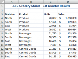
Excel Data Set

Data Set in Excel

Many people are curious about Excel Pivot Tables. They would like to learn how to create a Pivot Table, but they fear that that will take too long and be difficult to learn. 

Here’s the good news! Pivot Tables are one of the most powerful tool in Excel AND Pivot Tables are also one of the easiest Excel Techniques to learn! It sounds like a contradiction, doesn’t it? 

How would you like to turn this data set – with over 500 rows of data … 

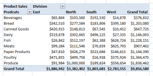
into this Pivot Table Summary Report with @ six clicks of the mouse? 

Pivot Table Row & Column

Pivot Table Summary

 That’s all it takes. With a Pivot Table you turn long lists of data into summarized information that highlights the trends and patterns in your business. 

Special: Save 20% on any purchase! Use Coupon SAVE-20-PCT during Checkout! 

I can teach you how to get started on the road to mastering Excel Pivot Tables. On my DVD-ROM, “The 50 Best Tips for Excel 2007,” I have the following Pivot Table video lessons: 

  • Introducing Pivot Tables – Run time: 8:23
    • Why Use Pivot Tables?
    • How to Create a Pivot Table
    • How to Modify a Pivot Table
    • How to Update a Pivot Table
  • Grouping and Charting in Pivot Tables – Run time: 5:50
    • Grouping Pivot Table Fields by Month, Quarter and Year
    • Grouping Pivot Table Fields by Week
    • Collapsing and Expanding Pivot Table Fields
    • Creating Pivot Charts
  • Using New Pivot Table Features in Excel 2007 – Run time: 7:46
    • Base Your Pivot Table on an Excel Table
    • Adjust Pivot Table Report Layouts
    • Apply Conditional Formatting to Pivot Tables
    • Insert Blank Rows in Your Pivot Table Report
The 50 Best Tips

The 50 Best Tips Series

As you can see from the “Run times,” each lesson is focused on one Excel technique. If you don’t have a lot of time and you want to quickly learn how to create Pivot Tables, my DVD-ROM is the best place to begin. 

Here is a PDF that you can download to see the content and Run times for each of my tips: The 50 Best Tips for Excel 2007 Detailed Content Listing 

And, here is a link to my Archive of Free Pivot Table Videos  on The Company Rocks website. 

Learn how to “Quickly Create Excel Pivot Table Reports and Charts” 

Thank you! 

Danny Rocks

The 50 Best Tips for Excel 2007 – Download Detailed Content Listing

By request, I have created a detailed content listing of each of “The 50 Best Tips for Excel 2007” available for you to download. Not only do you get a List of the 50 Best Tips, you also get details of the learning points in each tip and the Run time for each video lesson.  

Excel Tip List

Excel DVD Tips

You can download: 

If you would like to receive this detailed content listing as an Excel File, please click on this link to contact me directly. I will email you the file as an attachment. 

There are over 5 1/2 hours of focused video instruction on my DVD-ROM.The files are Shockwave Flash Files and they play in any Internet Browser (Internet Explorer, FireFox,Safari, etc.) 

As a bonus, the DVD-ROM contains the 50 Excel Workbooks that I use in the video lessons. Use these workbooks to recreate the lessons that you learn on the video. 

I invite you to visit my online store ( http://shop.thecompanyrocks.com) to purchase the DVD-ROM for “The 50 Best Tips for Excel 2007.” Click here to start shopping using my secure shopping cart. I guarantee your complete satisfaction with my products. If you are not satisfied, I will refund your purchase price with no questions asked. 

You will learn how to “Master Excel in Minutes – Not Months!”

Sincerely, 

Danny Rocks

Using the Built-in Excel Data Form to Edit, Enter and View Records

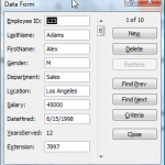
Data Form in Excel

Data Form

Excel has a built-in Data Form which is very useful for viewing all of the fields (up to 32 of them) associated with a single record. When you have lots of “Fields” in your “Data Set” and you do not want to do a lot of horizontal scrolling to view or edit the values in the cells, use this Data Form.

There is a limit of 32 fields when using Excel’s built-in Data Form.

Customize the Quick Access Toolbar

However, it does not appear as a Ribbon Command in Excel 2007. To use the Data Form add the Form Command to your Quick Access Toolbar (QAT) – I show you how to do this in the video.

Personally, I do not recommend the Excel Data Form for entering new records in your data set. I like to add Data Validation drop-down lists to ensure data integrity and this feature is not available in the Data Form. However, you can use Criteria to quickly find records for viewing and editing in the form.

Filtering Data with the Data Form

I give you a brief introduction to some of the new filtering options available in Excel 2007. I will cover this in greater detail in another lesson.

Subscribe to My Video Podcast on iTunes

I invite you to subscribe to my free video podcast, “Danny Rocks Tips and Timesavers” on iTunes. Click here to go directly to my iTunes podcast. I have had over 25,000 downloads since I began my podcast in June of 2010.

Watch this video in High Definition

Click here to go to my DannyRocksExcels YouTube Channel.

Watch Video Now

Master Excel in Minutes Video Training Resources

I have created a series of extended length Excel Video Training Resources. I invite you to visit my secure online shopping site to: Learn how to “Master Excel in Minutes – Not Months!”