Video Lessons For Excel | The Company Rocks

Danny December 30, 2009 Leave a Comment

The Online Store for The Company Rocks has Opened for Business!

I am proud to announce that my online store for The Company Rocks is now open!

You can now purchase my two DVDs without leaving my website.

“The 50 Best Tips for Excel 2007” contains over 5 1/2 hours of training. Each video lesson focuses on one tip and you can learn it in @ 6 minutes! The tips range from Beginning Level to the Advanced level. The majority of Tips (30 tips) are at the Intermediate level. If you enjoy the lessons that I post here, now you can own a DVD of the 50 Best Tips – now for Excel 2007!

“The 50 Best Tips for PowerPoint 2007” contains over 7 hours of training on two DVDs! I put a lot of effort into producing this DVD – and the customers who have already purchased it tell me that has immediately improved their presentation skills.

This DVD is unique!

Because, I do not teach PowerPoint as a “techie.” Rather, I am a professional speaker and trainer and I show you how to use PowerPoint as a tool to use during your presentations. Of course I show you how to create animations and how to create custom PowerPoint shows. But, significantly, I demonstrate how best to use custom animations and why you should prepare Custom PowerPoint shows. If you think you know PowerPoint, think again. I guarantee that you will learn new techniques for PowerPoint and … you will learn how to take advantage of the many great new graphic features available in PowerPoint 2007.

I invite you to visit my online store. The DVDs are in stock and attractively priced. I know that you will learn new tips and refine your skills in PowerPoint and Excel when you watch one of my lessons.

Invest 10 minutes to learn a new productivity tip – and, save yourself hours of frustration and avoid having to rekey data entries in Excel 2007.
Invest 10 minutes to learn a new presentation tip – and, learn how to deliver presentations using PowerPoint 2007 that get you the sale or get your audience to take action.
Invest 10 minutes and learn how to use the new Office 2007 interface. I show you how to always have your favorite commands right at your fingertips.

Finally, let me wish you a very Happy New Year in 2010!

Sincerely,

Danny Rocks

danny@thecompanyrocks.com

Danny October 30, 2009 Leave a Comment

Calculate the Days Worked on a Project

Do you manage Projects? Do you create Project work schedules? Do you need to know how many days were actually worked on your Project?

If so, this Excel video lesson is for you. A viewer asked for my help. He did not want to use MS Project for his work schedules. Rather, he wants to know which Excel Functions to use for his Project work schedules.

Excel Functions Covered in this Tutorial

In this lesson, I demonstrate how to use two functions included in the Excel “Analysis Tool-Pak”:

=WORKDAY()
=NETWORKDAYS()

Index of Excel Video Tutorials

Search for a specific Excel Video Lesson on this website in my Index.

Watch Excel Tutorial on YouTube

Click on this link to watch this Excel Tutorial on my YouTube Channel – DannyRocksExcels

Secure Online Shopping for My Resources

Want to learn how to get the most out of Excel 2007?

My DVD, “The 50 Best Tips, Tricks & Techniques for Excel 2007” is available for purchase.

Filed Under: Excel Date and Time Functions, Excel Financial Tools, Excel Functions, Excel Training, Video Response to Viewers Tagged: Excel Add-ins, Excel Video Training, Named Cells and Ranges, NETWORKDAYS Function, Project Estimates, project management, Video lessons for Excel, WORKDAY Function

Danny October 18, 2009 Leave a Comment

Use the Transpose Feature to Change the Orientation of Data Imported into Excel

I am working through the special requests that viewers have sent me. In this lesson, I show you how to:

Use Data – Get External Data – to import a simple delimited text file.
Use Copy – Paste Special – Transpose – to make a copy of the imported data that is now “vertically oriented.” i.e. The field entries run down the column rather than across the rows.
Use the Data – Text-to-Columns feature to break an “address block” (City, State, Zip Code) that is one cell into three distinct cells. This is a terrific time saver!

Now available for purchase: My DVD “The 50 Best Tips, Tricks, and Techniques for Excel 2007”

Over 5 1/2 hours of training. Each video lesson focuses on one tip and averages 6 minutes.

Now available from the online store at www.thecompanyrocks.com

Three Frustrations When Calculating TIme in Excel

When I am training a class to use MS Excel, I always get at least one question about performing time calculations. I sense that the person asking the question is frustrated. When I ask, “How many of you are frustrated when you try to perform a calculation to total time periods in Excel?” nearly every hand is raised! And they are right; Excel’s time calculations can cause frustration.

In this video lesson, I will show you how to overcome three common frustrations that you may have when performing time calculations in Excel.

Here are the steps to follow in this Excel Training Video:

Format the cell that contains the formula =End_Time – Start_Time) to the Custom Number Format h:mm
I encourage you to use this formula instead of a simple formula: =IF(End_Time < Start_Time, End_Time + 1, End_Time)-Start_Time.
This will eliminate any possible “Negative times” which result in a cell filled with ######### A Negative Time is frequently the result of “Time Periods that Span Midnight. e.g. Start @ 11:00 PM and End @ 3:00 AM
TIP: Use this Formula =MOD(End_Time – Start_Time, 1) This is the MODULUS Function.
When you calculate the total number of hours and the result exceeds 24 hours, use this Format [h]:mm

Search My Index of Excel Video Lessons

“The 50 Best Tips for …” is now available at the online store for The Company Rocks

How to Create a Combination Chart in Excel

What is a Combination Chart? When do I use one? Why do I use one?

What: A combination chart uses two different chart types in the same graphic representation of your data.
When: There is a large value gap between one data series and the other data series.
Why: To reveal the relationships in your data that may not be apparent with a traditional chart or by merely examining the data.

In this short video lesson, I will demonstrate “How” to transform a traditional column chart into a Combination Chart that reveals an interesting data relationship.

Here are the steps to follow in this Excel Video Lesson:

Start with a standard Excel Chart – Here we used the F11 Key to create a Column Chart in a separate worksheet.
Notice the wide gap between the two data series. Click on one of the series columns (in this case “Dollars”) and on the Chart Toolbar select the “Line” chart type.
A wide gap in values remains between the two series. With the “Dollars” series selected, choose Format Series on the Toolbar. Click the Axis Tab and select “Plot Series on Secondary Axis.”
Format the chart to suit your needs. In this example, we change the color of the Plot Area and add Text to a “Call out” shape on the chart.

Find the Excel Video Lesson that you want. Index of all Excel Topics

News! My DVD, “The 50 Best Tips for Excel 2007” is now available to purchase. I invite you to visit my online bookstore for more details.

My 5-Star Excel Video Lessons on YouTube

YouTube Logo

I have posted several of my MS Excel 2003 Video Lessons on YouTube. The YouTube community votes or rates individual videos. I’d like to share the results with you. To make it easy for you to view a video that interests you, I have established “Hyperlinks” to take you directly to that video lesson. Simply click on the title and you can view the tutorial.

Here is a listing of my 5-Star Excel Videos on You Tube:

News! My DVD, “The 50 Best Tips for Excel 2007” is now availabe to purchase. I invite you to visit my online bookstore for more details.

Filed Under: Excel Training, Most Viewed Excel Videos, YouTube Videos by Danny Rocks Tagged: 5-Star Rated Videos on YouTube, Excel Video Training, Free MS Excel Video Lessons, Hyperlinks, Video lessons for Excel

Danny September 5, 2008 2 Comments

Excel 2003 Basics – Data Entry

A viewer wrote in to request a few videos that cover “The Basics” in Excel 2003. In this video lesson, I cover the basics of data entry.

Even if you have been using Excel for a number of years, I guarantee that you will pick up one or two tips in this video that will save you time and make you more productive.

Here are the steps to follow in this video lesson:

Excel aligns “text” entries to the left-side of the cell. “Numeric” entries (including Dates & Times) are aligned to the right-side of the cell.
All calculations in Excel MUST start with the =sign. This includes Formulas and Functions. Write formulas that refer to other cells. (Avoid writing formulas that only use constant values.)
When we input data in a cell and press the ENTER key, Excel accepts the entry and makes the cell that is down one row in the column the “Active Cell.”
To input data in the cells of the same row – and continue to use the ENTER key – first select the range of cells in the row.
You can also select a range of cells in adjacent rows and columns. Excel goes down the cells in the column first and then moves automatically to the top row in the next column in your selection.

News! My DVD, “The 50 Best Tips for Excel 2007” is now availabe to purchase. I invite you to visit my online bookstore for more details.

Find the Excel Video Lesson that you want – Index to all Excel Topics

Filed Under: Excel Basics, Excel Training Tagged: Data alignment in cells, Dates and Times in Excel, Excel Video Training, Use the Enter key to input data across a row, Video lessons for Excel

Danny August 24, 2008 3 Comments

Create a Calculated Field in Your Pivot Table

When someone wants to see an additional field in your Pivot Table – e.g. to show the “Price per Units Sold,” you create a “Calculated Field.” This is a fairly simple process. In this video, Danny will show you how. This is yet another example of how you can use the power of a Pivot Table to present data the way that you – or your audience – want to see it.

Here are the steps to follow in this lesson:

On the Pivot Table drop-down menu select “Formulas, Calculated Field.”
In the dialog box, write in a Name for your new Calculated Field.
Enter the Formula. Use the Fields in your Pivot Table and any operators (+,-,*,/) Click OK.
Use the Field Settings to change any formatting, etc.

Find the Excel Training Video you want

Index to all Excel Topics

My DVD, “The 50 Best Tips for Excel 2007” is now availabe to purchase. I invite you to visit my online bookstore for more details.

Get a Free 28 Minute Excel Video Tutorial

Follow this link for information to download – “Introduction to Pivot Tables in Excel 2003”

Filed Under: Excel Training, Pivot Tables Tagged: Calculated Fields in Pivot Tables, Excel Pivot Tables, Excel Video Training, Video lessons for Excel

Danny August 22, 2008 16 Comments

Use Pivot Tables to Summarize by Year, Quarter and Month

Can you imagine trying to use Excel Subtotals to summarize a long column sales – listed by date? What would you subtotal? At every change in date?

This would be a nightmare! This would produce a useless report!

Pivot Tables, on the other hand, can provide a summary of dates by month, quarter, and year with just a few mouse clicks!

In this video lesson I show you how to produce that summary. The Pivot Table will transform a long list of data into information that you can use to analyze trends.

Here are the steps to follow in this lesson:

Create a Pivot Table using all of the default settings. Drag the “Date” field into the ROW area and the “Sales” field into the DATA area of the Template.
With 1 cell in the “Date” row selected, choose “Group & Show Detail, Group.” Select Year, Quarter and Month and click OK.
You now have 3 ROWS in your Pivot Table – Year, Quarter & Month. Drag the Year field from the ROW up to the COLUMN area. Hide on of the “Grand Totals.”
Click the Pivot Chart icon to create a Pivot Chart on a new worksheet. Filter the data fields.
Move the Year field back to the Row area. Ungroup the fields to return to the starting point.
To Group by WEEK: Choose “Group & Show Detail, Group” and select DAY. Then select 7 for the number of days in the week.

Find the Excel Training Video that you want – Index of all Excel Topics

Additional Pivot Table Resources

Pivot Table Training Resources

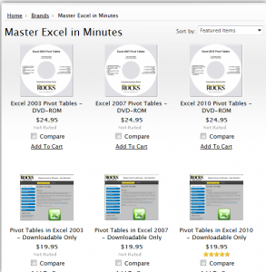
I have published a 90 minute focused video tutorial for Pivot Tables. It is available for each version of Excel -2010, 2007, and 2003. You can purchase it as either a DVD-ROM that I will ship to you or as a Downloadable version that you can work with immediately.

In addition to the 90 minutes of video instruction on Pivot Tables, the package includes:

The Excel Practice Files that I used while filming the video tutorial – so that you can practice your new skills using the same files that are on the video.

I invite you to visit my secure online shopping website – http://shop.thecompanyrocks.com – to learn about the many training resources that I offer for sale.

A Step-by-step Instructional Guide that you can print out – so that you can use it to take notes as you watch my video tutorial.

Danny Rocks “Training You to Excel”

The Online Store for The Company Rocks has Opened for Business!